
Externalities, Pigouvian Taxation, and Optimal Policy
Are Pigouvian Taxes Actually Optimal Solutions to Externalities?

Here at Economic Forces, we love writing about externalities. They are fun to write about. On some level, they seem really easy to understand. Introductory textbooks certainly make them seem easy. Yet, this simplicity is illusory. Externalities are quite complicated.
The way that externalities are typically taught at the introductory level is as follows. A negative externality is a cost paid by a third party to normal market activity that is not reflected in the price of the good being traded. As a result, the social cost is greater than the private cost. Because this cost is not paid by market participants, no one internalizes the cost and the resulting equilibrium quantity is inefficiently high. The standard textbook argument is that the government should levy a tax on this activity equal to the marginal external cost (the difference between the marginal social cost and the marginal private cost). This tax is referred to as a Pigouvian tax. By doing so, this forces market participants to internalize the cost. The resulting equilibrium quantity in the market is the socially efficient quantity.
But is this policy really optimal? If so, in what sense? If not, why not?
Setting the Stage
Let’s imagine that there are 3 distinct groups. There are consumers, producers, and those who are not in the market at all but who suffer the external costs. Let’s assume that all costs are variable and the cost of production and the external cost are both linear in quantity. This implies that both the marginal cost of production and the marginal external cost are constant and equal to the average cost of production and the average external cost, respectively. The market is competitive and the supply curve is horizontal.
As any student of introductory economics knows, a tax drives a wedge between the price that buyers pay and the price that sellers receive. Since the supply curve is horizontal, the entire area to the left of the demand curve due to this tax wedge is a reduction in consumer surplus. Some of this area goes to the government in the form of tax revenue. The remainder is the excess burden, or deadweight loss, of the tax.
If the size of the tax is equal to the marginal external cost, this does in fact reduce the quantity traded to the amount that the market would choose if all the costs were internalized. This is often referred to as the efficient quantity.
Nonetheless, it is important to note that the consumer is worse off. This is true even if the tax revenue is used to make a lump sum transfer to the consumers, or otherwise paid to them in a way that doesn’t affect their choice in the relevant market we are discussing. The reason for this is that the total reduction in the consumer surplus is greater than the tax revenue.
It follows that the Pigouvian tax is not Pareto improving since consumers are worse off.
An Alternative Framework
Pigou wasn’t the only economist famously known for thinking about externalities. Ronald Coase is also famous for thinking about the problems of social cost. Coase emphasized property rights. These external costs we’ve been referencing often follow from an incomplete definition of property rights. For example, a frequently used example of a negative externality is a factory that pollutes a river upstream from a fishery. If either the fishery or the factory are assigned the property rights to the river, then the two parties could negotiate. For example, if the fishery is assigned property rights to the river, the fishery could prevent the factory from polluting the river unless the factory offers sufficient compensation to the fishery. That compensation forces the factory to internalize the cost of its pollution. Alternatively, if the property rights to the river are assigned to the factory, the fishery could pay the factory to limit its production in order reduce pollution.
Ideally, it would be great to be able to compare Pigouvian taxes to Coaseian logic within one coherent framework. Fortunately, the new edition of Chicago Price Theory contains an example that does just that. It requires thinking about demand a bit differently.
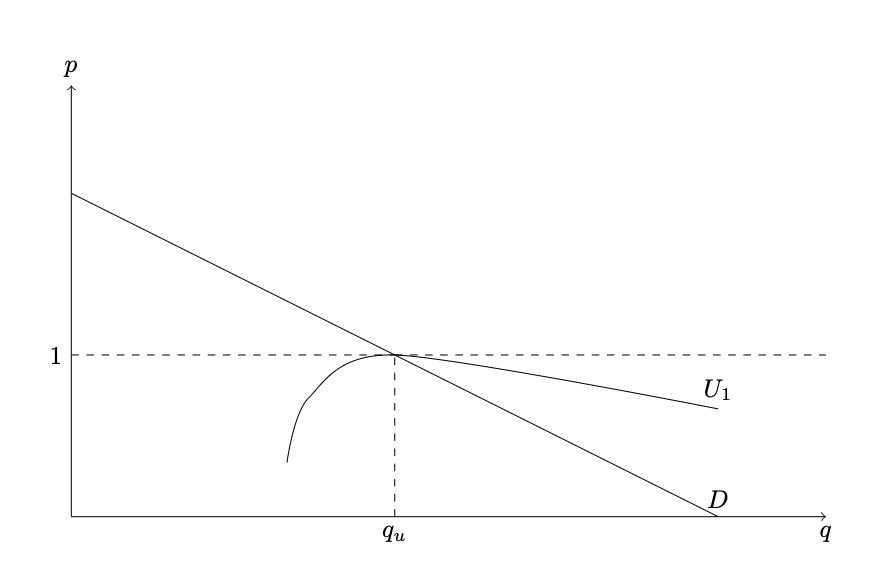
Consider the following example. Suppose that we have a demand curve as depicted in the figure below. The demand curve shows the typical negative relationship between price and quantity demanded. A tool that Kevin Murphy likes to use is to draw indifference curves in the price and quantity space. But what would an indifference curve look like in this context? As depicted in the figure below, for the price equal to 1, one can draw and indifference curve that is tangent to a horizontal line consistent with the price. Near this price, the indifference curve is relatively flat. This is because consumers are pretty indifferent about the quantity around the given price. They’ll take a little higher or a little lower quantity at a slightly lower price and be just as content as they are with the quantity demanded associated with a price of 1. The indifference curve is pretty steep to the left of the demand curve. This is because as the quantity the consumer gets to consumer declines, the consumer has to be compensated with a lower and lower price to keep them just as well off. To the right of the demand curve, the indifference curve is relatively flat because the consumer doesn’t need a much lower price to consume a little more.
Note that this also implies that lower indifference curves are preferred by consumers on this figure. This is because for a given quantity, the consumer prefers a lower price.
Now, let’s suppose that marginal private cost is 1 and the marginal social cost is
The figure below shows that quantity that would be chosen in the absence of a Pigouvian tax would indeed be q_u. A Pigouvian tax equal to the marginal external cost would result in the equilibrium quantity, q_e. This is the quantity demanded when consumers must pay the marginal social cost and is therefore the efficient quantity of output in the market.
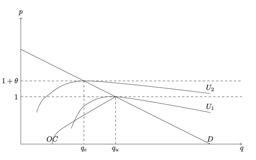
Given what we know about the indifference curves plotted in price and quantity space, it is straightforward to see from this second graph that a Pigouvian tax makes the consumer worse off. This is a different way of illustrating the point I discussed above. A Pigouvian tax can make sure that the equilibrium quantity of output is efficient, but the tax isn’t Pareto optimal. In order for the tax to be Pareto improving, it would need to make some people better off without making others worse off. However, it clearly makes consumers worse off.
This begs the question: Is there a way to make sure that the efficient quantity is the equilibrium outcome while simultaneously being a Pareto improvement?
In order to think about this, we need to think about the welfare of the other people in the market, producers and those outside the market who suffer the costs of the externality. For simplicity, let’s lump both these groups together. In addition, let’s think of this group’s welfare as equivalent to the total surplus to the group. We can define the “other surplus” that goes to others in the market as follows:
Where the total surplus is the combined surplus to producers minus the external cost to those outside the market. To think about how this can be illustrated on our graph, consider the following example. Suppose that the marginal external cost is 1/2. It is possible to think about combinations of p and q that provide the same surplus. To see, why let’s consider some examples. Imagine that when the p = 1, q_u = 48. This implies the surplus is -24. Now, consider that if the price is 1/2, the quantity that provides the same amount of surplus is 24. If the price is 3/10, the quantity that yields the same surplus is 20. If the price is 0, the quantity that produces the same surplus is 16. Thus, one can illustrate the “other surplus” in the figure as the curve OC.
Now, we are prepared to think in Coaseian terms. Note that for any given quantity, the “other surplus” is increasing in p. It follows that any point above the line denoted OC, the combined group of producers and those who suffer the cost of the externality are better off. At the same time, we know that any point that lies below U_1 makes consumers better off. It must therefore be true that the area between the indifference curve labeled U_1 and the OC curve represents potential gains from trade between the consumers and the others.
The Pareto optimum solution is achieved at the point at which the others’ surplus curve is tangent to the consumer’s indifference curve. Consider the following example. For the OC curve as it is drawn, a lower indifference curve tangent to the OC curve would make consumers better office without making the others worse off. The tangency point between these two curves is a Pareto optimal outcome because in comparison to that tangency point, there is no other point that can make one group better off without making the other group worse off.
It is also important to note from the graph that there are many points on the graph between U_1 and OC associated with the efficient quantity. This not only tells us that the efficient outcome is possible, but that we can get to the efficient outcome without the Pigouvian tax and in a way that consumers would prefer to the Pigouvian tax.
Of course, there are a couple of things to note here. The efficient outcome is not possible if the marginal price is set below 1. If the marginal price is uniform to all consumers and set below 1, the quantity demanded would be even greater than q_u. Implementing the efficient equilibrium outcome without Pigouvian taxation would require that the marginal price is greater than 1 and the average price is less than 1. This entails some non-linear pricing scheme.
To turn this back to Coase, there might be some voluntary solution via bargaining that implements a non-linear pricing scheme that is Pareto improving. This would likely require setting up some type of organization that can impose this type of non-linear pricing in order to generate a Pareto-improving outcome.
Whether or not the efficient quantity can be achieved and how close such an organization can get to the efficient quantity depends on cooperation costs. As Coase alluded to with regards to transaction costs more broadly, coordination costs limit the ability to achieve the efficient outcome.
Some Concluding Thoughts
The standard argument that negative externalities can dealt with by implementing a Pigouvian tax ignore some of the welfare implications of the tax. Such taxes might produce the socially efficient quantity, but these taxes are not Pareto improving.
In fact, externalities are substantially more complicated if we take Pareto optimality seriously. The Coaseian logic that bargaining can produce a better outcome is illustrated by thinking about the total surplus from trade of all parties involved, including those who bear the external costs. Furthermore, as Coase himself emphasized, the ability to reach the efficient outcome through a voluntary solution is limited by transaction (in this case, coordination) costs.
This is just one more example of why we spend so much time on externalities here at Economic Forces. The average introductory textbook often makes externalities seem straightforward and the policy solutions seem easy. When it comes to providing caveats to the Pigouvian policy solution, textbooks might acknowledge the difficulty of estimating the true marginal external cost. Some textbooks might even mention that there can be a tension between the Pigouvian tax that implements the efficient quantity of output and the Pigouvian tax that generates the most revenue. Nonetheless, this is only part of the story. A bigger limitation is that Pigouvian taxation isn’t Pareto-improving.
If you want the efficient quantity of output and you want to make sure there is a Pareto improvement, a Pigouvian tax simply won’t do.
In the real world, the "producer" category is not a monolith. Certain businesses actively lobby for Pigouvian taxes to gain a competitive edge:
Firms that already utilize clean energy or sustainable methods will push for carbon or pollution taxes. The tax artificially raises the costs of their dirty-tech competitors, driving those rivals out of business.
Massive corporations sometimes weaponize Pigouvian taxes as a barrier to entry. A large firm can absorb the compliance and administrative costs of the tax, while smaller startups cannot and are forced to close.
So the answer is always transaction costs.