The invisible hand screws up your regression

Markets, diff-in-diff, and "The Missing Intercept" problem

You’ve probably heard the claim: “Chinese imports destroyed millions of American manufacturing jobs.”

Most likely, that number comes from the famous “China Shock” research by David Autor, David Dorn, and Gordon Hanson. It’s become a fixture in trade debates. In that original paper, Autor, Dorn, and Hanson compared regions with different exposure to Chinese import competition. Some areas manufactured goods that competed directly with Chinese imports. Others didn’t. By comparing employment changes across these regions, the researchers identified how relative employment shifted; high-exposure regions lost jobs compared to low-exposure regions.

In a benchmarking calculation, they estimate that Chinese import competition accounts for approximately 21% of the U.S. manufacturing employment decline from 1990 to 2007, corresponding to roughly 1.5 million manufacturing jobs.

How seriously should we take that number? Answering that question is actually quite informative for answering many issues in empirical economics.

Price theory makes empirical work hard

One of the core premises of price theory is that prices coordinate people. Firms don’t exist in isolation; they’re competing with other firms. When Honda’s costs rise, it may produce less, which affects the demand for Toyotas. Firms are also connected across markets. They buy inputs from other firms, sell outputs to consumers and other firms, and compete for workers with every other employer in the economy.

Because prices coordinate behavior across all participants, when you shock one part of the system, the price mechanism transmits that shock everywhere else. Wages adjust. Workers relocate. Capital flows to different uses. Industries expand and contract.

This is an eternal nightmare for empirical work in economics. We rarely observe a clean experiment where only one thing changes. We see the whole interconnected mess moving together. Clever identification strategies try to isolate specific causal effects by finding variation that hits some units but not others. That’s valuable. But it also means we’re often measuring something specific: how the treated units changed relative to the untreated units.

And that’s not always what we want to know.

Robert Minton and Casey Mulligan have been developing what they call a “market interpretation of treatment effects” that clarifies what’s happening here. Their key insight is the simple idea above: in markets, prices coordinate behavior across all participants. When you shock one part of the market, the price system transmits that shock everywhere. The control group is RARELY unaffected. The treatment spills over onto them.

Their framework distinguishes three things that people often confuse:

• Difference-in-Differences (DiD): The gap between the treated and the controls. This is what your standard regression estimates.

• Treatment on the Treated (ToT): What happened to the treated compared to the baseline. This includes any spillover effects.

• Scale Effect: What happens when you treat the entire market. This is often what policymakers actually care about.

These three are not the same thing. Usually, when we talk about spillovers, economists will point to a small treatment size, meaning spillovers are small. But ToT and DiD become less informative about the scale effect as the share of treated units falls. In the limit of a tiny treated share, ToT and DiD coincide with each other (which is often what microeconomists want) but can differ from the scale effect by an arbitrary amount (which is often what the public discussion is about).

Before getting into the details, let’s think about the intuition for why these are different. You’re at a concert. You stand up to see better. The person behind you is now blocked, so they see worse.

A researcher measures the difference: “Standing up improves your view by X relative to the person behind you.” Correct! Now the researcher scales up: “If everyone stands up, everyone will see better by X.” Obviously wrong. If everyone stands up, nobody sees better, and everyone just has tired legs.

Econometricians have long grappled with spillovers or externalities, but more as a complication.

As Minton and Mulligan point out, this is the norm in markets. They illustrate this with a simple industry model that makes the problem precise.

Start at the market level. You have a downward-sloping demand curve and an upward-sloping supply curve. In the baseline, before any treatment, the market clears at some equilibrium price and quantity. Now imagine some suppliers get a productivity treatment so their output rises. The supply curve shifts outward. A new equilibrium emerges at a lower market price and higher total quantity, moving from E to E’ in the figure below. If the full market were treated, you’d move to E’’.

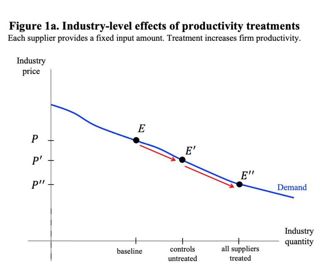
Now look at the firm level. In the baseline, treated and untreated firms have the same output and revenue. After the treatment, the treated firms can produce more. But the additional output from the treated drives down the market price that all suppliers receive. The untreated firms haven’t changed their production at all, but they now get paid less for every unit they sell.

After the treatment, the price is P’, so the treated firms receive revenue R_3 + R_4 + R_5 + R_6. The untreated firms have a revenue of R_3 + R_5. The DiD picks up the difference: R_4 + R_6.

If we ask what was the effect on the treated, we also have to account for the fact that prices fell from P to P’. The net effect on the treated is their new revenue (R_3 + R_4 + R_5 + R_6) minus their starting revenue (R_1 + R_3 + R_5). So ToT is R_4 + R_6 - R_1.

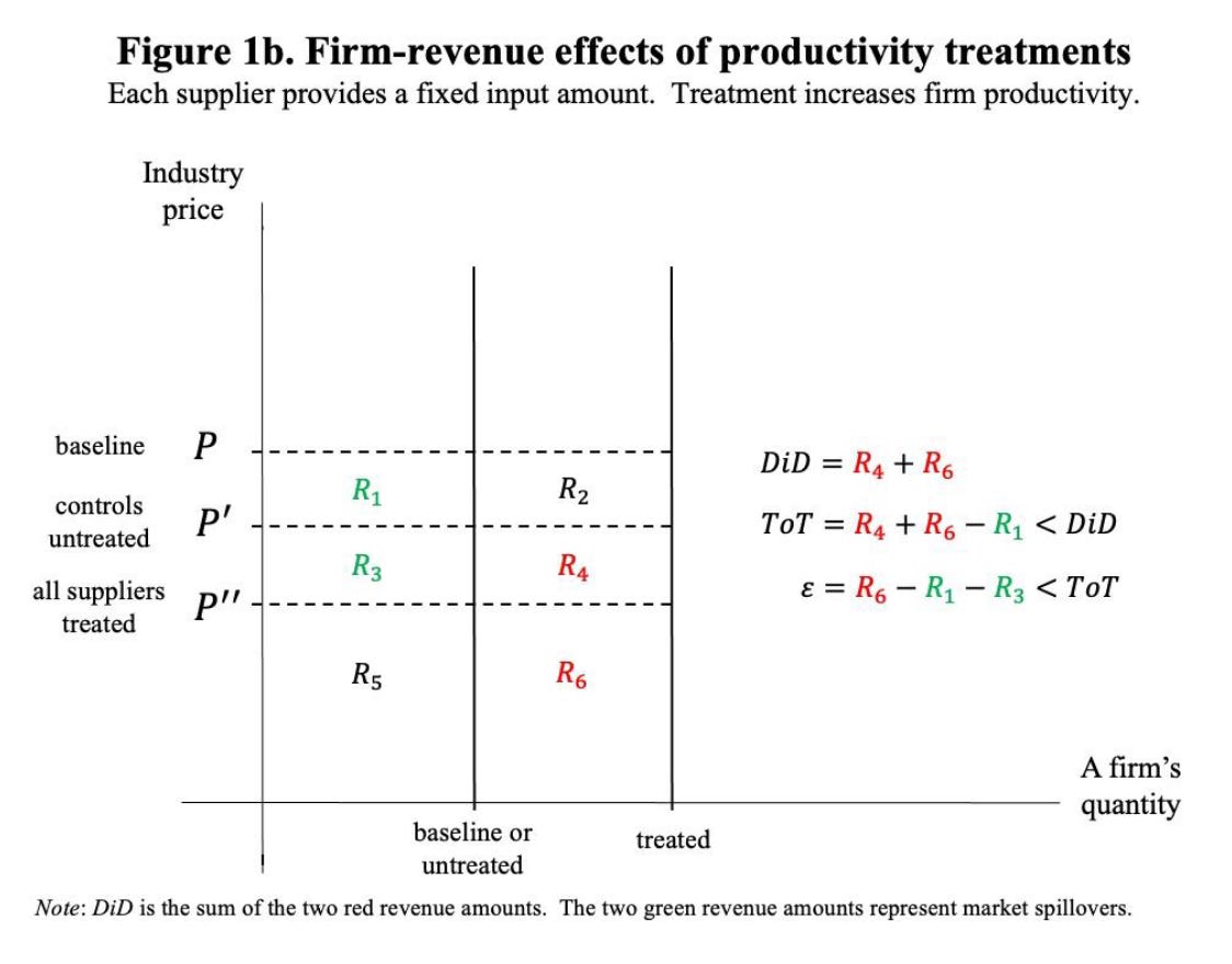
If we want to ask what would happen if all firms got the technology, now prices would go down to P’’. Revenue would go from R_1 + R_3 + R_5 to R_5 + R_6, so the net effect would be R_6 - R_1 - R_3, which is less than the ToT.

Notice what happened. DiD is positive (R_4 + R_6). But the scale effect (R_6 - R_1 - R_3) can be negative if R_1 + R_3 > R_6. That happens when demand is price inelastic, so that the price falls so much that even higher output doesn’t compensate.

A statistician might say the control group is “contaminated” because the treatment spills over through competition. But the contamination thinking doesn’t help us. For example, shrinking the treated share, which we generally think helps contamination issues, doesn’t fix this. The divergence between DiD and the scale effect persists no matter how small you make the treatment group. In fact, it gets worse: a smaller treated share means more of the market remains untreated, so the gap between “treating those we treated” and “treating everyone” grows larger.

The Missing Intercept

That’s the price theory framing. There’s an econometric way of seeing the same thing for the nerds who want that.

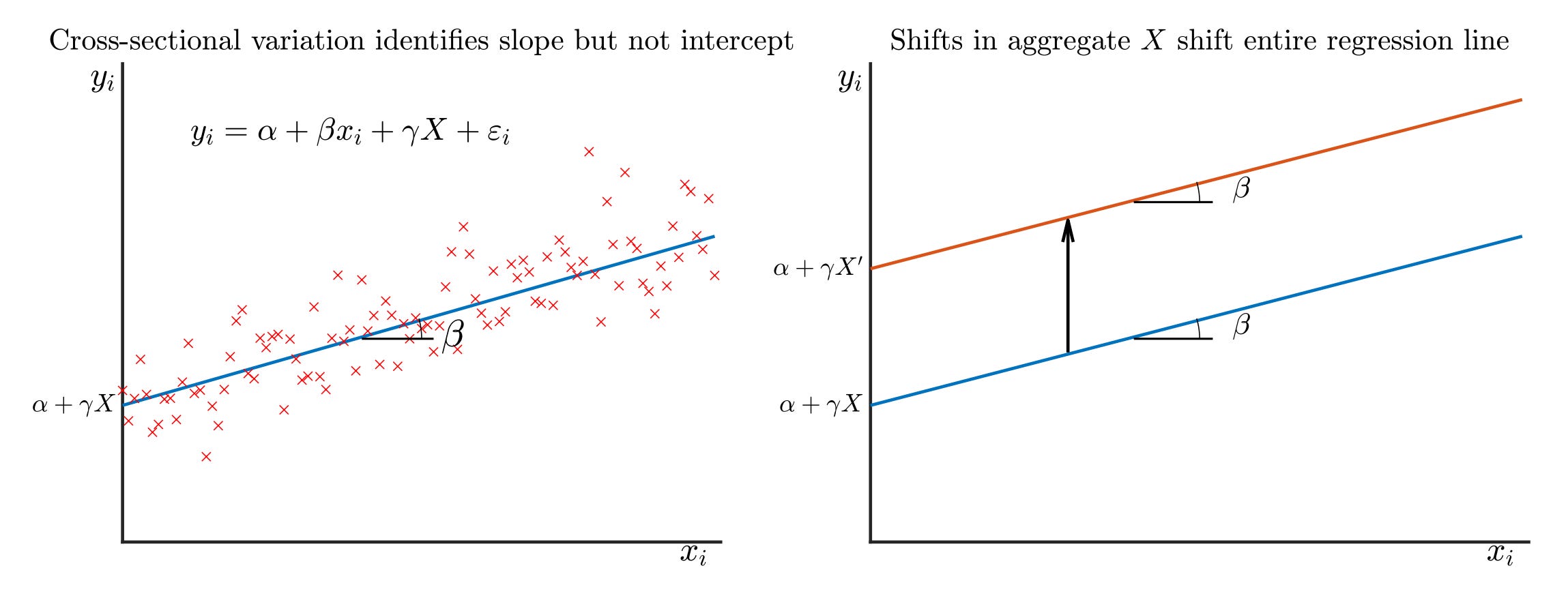
Your regression gives you a slope: how outcomes vary with treatment intensity across units. High-exposure regions lost more jobs than low-exposure regions. That slope is your DiD estimate.

The treatment effect on the treated isn’t just the gap between treated and controls. It’s that gap plus whatever happened to the controls because of the treatment. If competition from displaced manufacturing workers pushed down wages in services, that’s a spillover onto the “control” sector. The controls moved too.

So: ToT = DiD + the spillover onto controls.

Your regression identifies the slope. But that level shift—how much everyone moved because of the treatment—gets absorbed by the intercept (or maybe time fixed effects). It’s invisible to cross-sectional variation. Macro people sometimes call this the “missing intercept.” In Minton and Mulligan’s framing, it would be called the treatment effect on the untreated.

Notice that the scale effect is still different. ToT tells you what happened to the treated when you treated some of the market. The scale effect tells you what would happen if you treated all of it. The difference is the counterfactual spillover on the treated from additionally treating everyone else. When your treated group is small, that’s a lot of “everyone else.” The additional spillover can be large.

Formally, ToT is a weighted average of the scale effect and DiD. The weight depends on the fraction of the market that is treated. As that fraction shrinks toward zero, ToT converges to DiD, but both can differ from the scale effect by an arbitrary amount.

Two Distinct Problems

There are (at least) two conceptually different reasons you can’t just multiply the cross-sectional slope by aggregate treatment intensity to get the aggregate effect. Both matter in different proportions, depending on the problem.

Problem 1: Aggregate Shocks That Hit Everyone

At least in theory, some responses have literally zero cross-sectional variation. They hit everyone identically.

Did the Fed respond to rising unemployment by easing monetary policy? Did the dollar weaken? Did fiscal policy respond?

These affect everyone equally. Time fixed effects absorb them completely. Your regression cannot see them. There’s no cross-sectional variation to exploit.

Problem 2: Spillovers and Reallocation

When workers lose their jobs in one sector, they don’t vanish. They move—geographically or across industries—to find new work. They flood into other sectors.

The cross-sectional estimate captures substitution within the market. Basically, how activity shifted between treated and control groups. But some of that gap is zero-sum reshuffling that doesn’t affect the aggregate at all.

Minton and Mulligan push this further. Even if you could perfectly measure the spillovers—how much wages fell in the control sector when treated workers flooded in—you still wouldn’t recover the aggregate effect. The reason goes back to the distinction between ToT and the scale effect. Measuring spillovers onto controls gets you from DiD to ToT. But the scale effect is what happens when there’s no control sector left to absorb the shock.

If you want to know what happens when the entire economy is hit—when there’s no unaffected sector to flee to—you need a different elasticity entirely. Not the elasticity of substitution between the treated and control sectors, but the elasticity of substitution between working and not working. Between participating in this market and leaving it entirely.

The cross-sectional design identifies substitution within the market. The aggregate effect depends on substitution out of the market. These can be completely different numbers.

Back to the China Shock

Now we can return to that 1.5 million jobs number with clearer eyes.

The China Shock is different from the development economics case. When a development economist runs a microfinance pilot in a few villages, they may want to know: what would happen if we scaled this up nationally? That’s the scale effect question.

Autor, Dorn, and Hanson aren’t asking that. China has already happened to the whole economy. They’re trying to measure an aggregate shock that already occurred. The question is: what did Chinese imports actually do to American employment?

The problem is that they’re using cross-sectional variation to get at an aggregate effect. High-exposure regions lost jobs compared to low-exposure regions. That’s the DiD. Solid identification.

But to get the headline number, they multiply that regional slope by the national change in import penetration. Benjamin Moll calls this the “naive scale-up”:

Aggregate effect ≈ (micro coefficient) × (aggregate change in treatment)

This arithmetic looks innocent. But it goes against the basics of price theory. (To be fair, they recognize the problem and frame it as a benchmark.)

It assumes the aggregate effect is just DiD times the size of the shock. It assumes no spillovers, no reallocation, and no general equilibrium. This isn’t a secret in the paper, but it’s maybe missing by those who just casually know it.

What’s actually missing? The common component—how much everyone moved because of the China shock. Did displaced manufacturing workers flood into services, pushing down wages there? Did the Fed respond to rising unemployment? Did falling demand in factory towns hurt local retailers everywhere? These effects hit high-exposure and low-exposure regions together. They’re absorbed by time fixed effects. The cross-section can’t see them.

This is the “missing intercept” problem. It’s not that we want to know the intercept per se (when the treatment is zero) but that the research design identifies relative effects, or the slope. But the level shift that’s common to all regions disappears.

If manufacturing workers who lost their jobs moved into services, that displacement shows up as a huge gap between sectors, even if total employment barely changed. The DiD is large. The actual aggregate effect could be much smaller. Or if the common shock was large—if macro policy failed to respond, if there really was nowhere for workers to go—the aggregate effect could be larger than the cross-sectional estimate suggests.

I’m not saying the aggregate effect is zero. I’m saying the research design can’t tell us what it is. The naive scale-up assumes no spillovers. But the whole point of price theory is that spillovers are everywhere.

The Intercept Can Cut Either Way

I’ve been emphasizing what the cross-section misses. But I haven’t told you which direction it cuts. The missing intercept could make the aggregate effect smaller than the naive scale-up—or larger.

The cushioning intuition is natural. Workers displaced from manufacturing flood into services. The shock gets absorbed. The aggregate effect is smaller than the local one because there’s somewhere else to go.

But the intercept can also amplify.

Recent work by Adão, Arkolakis, and Esposito tries to recover the missing intercept using a structural general equilibrium model. They find that the China Shock eliminated 2.2 million jobs, a number even higher than the original estimate by Autor et al. In their model, regions are linked through trade and production chains. When a manufacturing hub shrinks due to import competition, it ceases to generate the agglomeration benefits that make nearby firms more productive.

On the other side, Lyon and Waugh incorporate aggregate labor supply responses, producing a positive aggregate employment effect from the China shock of about 1.5 million additional jobs. They explicitly state the limitation: difference-in-difference approaches identify only differential effects, not levels. The aggregate labor supply response is not identified. This is more about the aggregate shock that I mentioned above.

Now, I’m not claiming the 1.5 million number is too high. I’m not claiming it’s too low. Or I think it's below 1.5 million, but I’ll save sorting through that literature for another newsletter.

The point is that the research design of comparing high-exposure to low-exposure regions can’t adjudicate between these possibilities. The cross-section identifies the slope. The literature itself is an iterative attempt to reconstruct what cross-sectional designs omit. Even time variation is problematic. For example, Alessandria, Khan, Khederlarian, Ruhl, and Steinberg argue that the job losses we observed in the 2000s were largely the slow, grinding adjustment to earlier decisions. You can’t just difference that out. In a sense, the past is contaminating the WTO time period. Or in price theory language, this is markets interacting through time, not just across place.

Missing Intercepts Everywhere

I started out with how general this problem is. Yes, I tried to lure you in with the China shock number, but then it’s everywhere. The Moll slides that I linked about list a bunch of areas that fall prey to this. Let me add one more case where you need to worry about comparing treated and control groups: airline mergers.

Airline mergers have the "missing intercept" problem built in from the start.

The standard approach compares “treated” routes (where both merging carriers operated before) to “control” routes where only one carrier flew. Classic DiD.

But airlines operate networks. When Delta and Northwest merged, Delta didn’t just adjust fares on overlap routes. They reoptimized capacity, frequencies, and pricing across hundreds of routes. That’s the whole justification for the merger (maybe overblown, but still). Your “control” routes are connected to the treated routes through the network. They’re partially treated or contaminated.

Any common effect that hits all routes together, such as network-wide pricing changes, capacity discipline, or coordinated conduct, gets absorbed by time fixed effects. It’s invisible to the cross-sectional comparison. The DiD identifies the differential change between treated and control routes, not what happened to the overall level of fares.

A recent paper by Aryal, Chattopadhyaya, and Ciliberto is basically an attempt to grapple with these exact critiques. There are really two parts to their analysis. The first uses synthetic DiD to reweight controls to better match the pre-trends of the treated group. This addresses a parallel trends problem, a separate issue from the missing intercept. After this fix, the results shift dramatically. The baseline DiD suggests mergers reduced prices by 4-8%, but with synthetic weights, those effects vanish. If anything, prices rose.

But synthetic weights don’t solve the missing intercept problem. They ensure treated and control routes were on similar trajectories before the merger. They can’t tell you about common shocks that hit all routes together. If the merger generated efficiency gains that spread across the network, lowering prices on all routes, we wouldn’t pick that up. On the flip side, if the merger facilitated anticompetitive coordination across all routes, raising prices everywhere, we wouldn’t pick that up either. The intercept can cut either way.

The authors know this and are extremely clear about it. They explicitly flag that the standard merger DiD approach relies on no spillover effects across markets and note this is questionable when firms compete across markets.

That’s why the second part of their paper turns to a structural model, separately identifying efficiency gains and changes in “conduct.” This gives you a framework for thinking about what the missing intercept might contain. But the identification still comes from cross-sectional variation. The structure helps you interpret, but it doesn’t conjure new information from thin air.

So what are we to do? The authors try to rescue the analysis with a structural model, but I’m not sure it solves the fundamental problem. Novel methods in a single application should make us more cautious, not less. In the case of the airline mergers, I think this paper is the best we have on these mergers, and it looks like these mergers have raised prices.

But we should be quite humble at this point. The cross-sectional estimates require no-spillovers assumptions that are especially heroic for networked industries. The missing intercept problem is the norm when you’re dealing with networks.

The key point is that distributional effects and aggregate effects are different questions. Most of the time, the coefficient is a slope. The aggregate effect requires the slope and the intercept, which requires an economic model.

Markets connect people through prices. That’s what makes them so good at coordinating activity. It’s also what makes them so hard to study in pieces.