

Suppose there’s a seller who is (naturally) selling a good. As is the norm, if they lower the price, they would sell more of the good. This is sometimes called the monopoly model, but there’s nothing about monopoly that really matters here. How should the seller price the good?
Without solving the full optimal pricing problem, we know for sure that the seller won’t sell to everyone who values the good more than they do. This is the first thing we learn about. “Monopolies” restrict output. Nothing weird about this.
Now, let’s think of a slightly different situation. Instead of selling the good in a normal fixed-price setup, we’re in an auction room, and the seller has one object. Let’s assume they don’t care for it and it is worth nothing to them. There are two bidders who both value the good more than zero. Suppose A values it at $4 and B values it at $12. There is $12 of value in the room, the object is worth nothing to the seller, and if the seller wants the most money, the right move is to sell to neither of them. Refuse both bids.
How is that possible? I’m not pulling any tricks. I’m not assuming there is a second round. The auction ends, and everyone goes home, and the object stays unsold.
What I want to convince you of today is that this monopoly output restriction, which is week 3 stuff in Econ 101, is the same thing as the seemingly more complicated problem of the auctioneer.
More than that, sometimes the seller does sell, and sells to the bidder who values the object less. The high bidder goes home with nothing, and the low bidder walks out with the object. So we can’t summarize that as restricting output.
So what’s going on? That’s what this newsletter is about.
In a 1989 paper, Jeremy Bulow and John Roberts gave us the tools, which we will go through today. (Bulow has so many bangers.) There will be a little bit of notation and graphs along the way but no real math to worry about.

From values to demand curves
Let’s start with one buyer (not bidder yet). I’ll follow Bulow and Roberts’s numbers. A’s value is somewhere between 0 and 10. If we want to be precise, it’s drawn from a uniform distribution (each value is equally likely) between 0 and 10.
If the seller posts a price of $8, A will buy whenever his value exceeds $8, which happens 20% of the time. The seller has an expected revenue of $1.60. On the margin, lowering the price will attract bidder A when he values it below $8, but the seller will collect less when he values it above $8.
This generates the usual marginal revenue trade-off. How much do you get by trying to sell the product a little bit more? We’re used to thinking about selling one more unit of the good. Here since we have one good, we can think of the probability of sale and selling a bit more often.
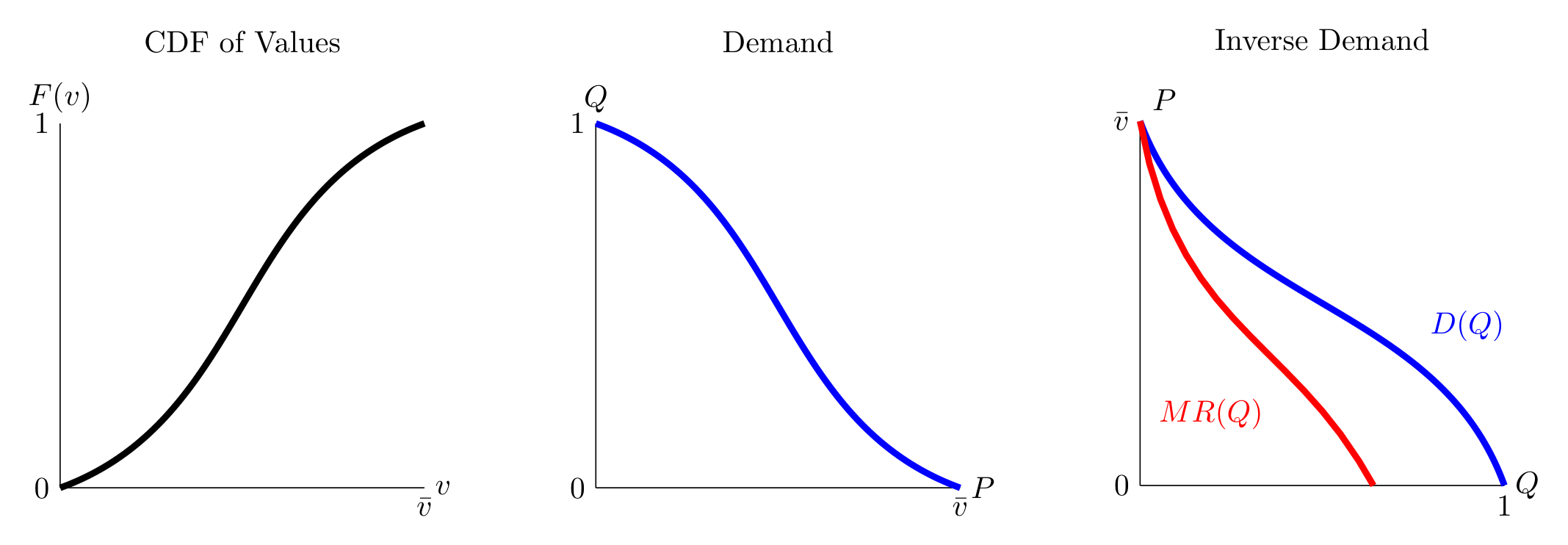
This is easier to visualize if we don’t have a uniform which is a straight line. More generally, if the bidder has a value from some cumulative distribution function (CDF of v), given by F(v), we can plot that on the left. If we imagine a posted price, this just flips to become the demand function (but with quantity on the y-axis). We can flip again to get our more standard inverse demand function.
If we think of a uniform distribution of values, this becomes the usual linear demand curve that we teach in Econ 101.
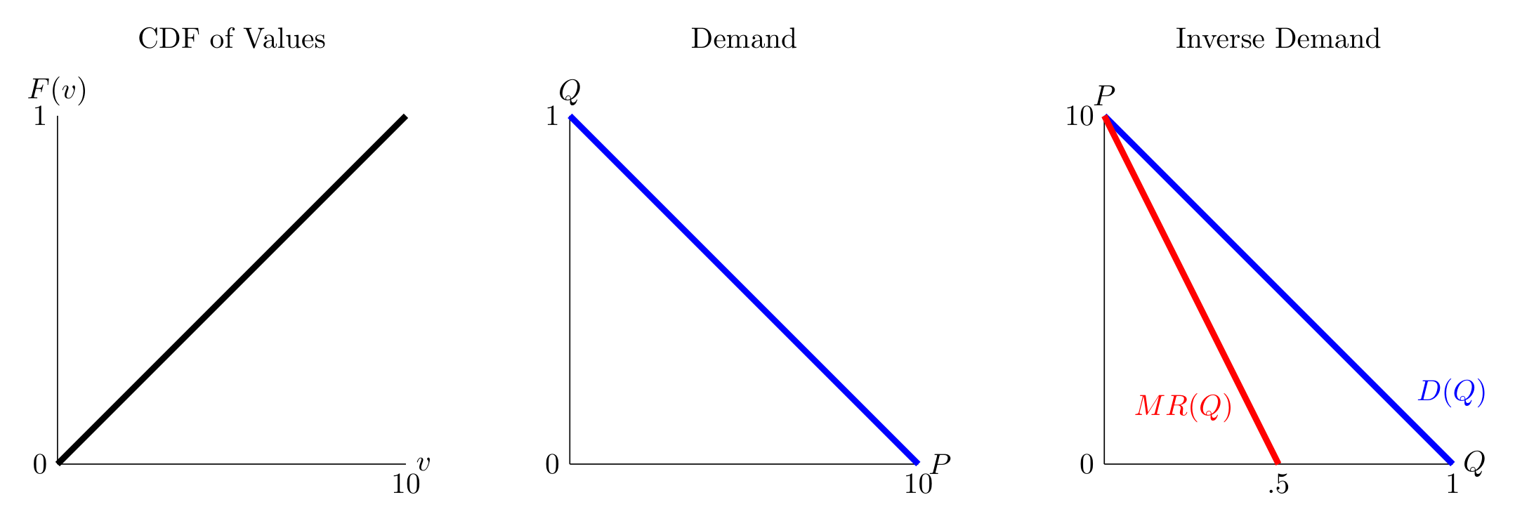
Bulow and Roberts show how that MR curve is what auction theory calls the virtual value.
Hard floors
Assume that you want to set some floor, a “hard floor.” You will not sell it to any bids below some price. Where do we find that? If you’d ask most people, maybe one idea would be to set it at the seller’s own value. That’d be the efficient thing to do, and you’d make sure that you always give it to somebody who values it more than the seller.
Let’s think about two bidders from the same distribution, uniform on (0,10). Let’s suppose we have a second-price auction with no reserve. That means people announce their bids, and the high bidder wins and pays the low bidder’s bid.
You can do better by setting a hard floor and refusing to sell below it. Suppose you set the floor at $5, which is where the MR curve hits zero, then traced up to the demand curve. It is the optimal floor to set, where the marginal revenue curve is zero.
Notice that my argument did not depend on how many bidders show up. The floor only matters in two different situations:
Nobody clears the floor, so there is no sale.
Exactly one bidder does, and they pay the floor.
In both of those cases, everyone else is below the floor and basically out of the picture. Whatever the number of bidders is, the seller in those situations is a one-bidder monopolist facing one demand curve, and sets the floor where that curve’s marginal revenue hits zero, $5. More bidders make those situations less common but they don’t change where the floor is.
Price discrimination
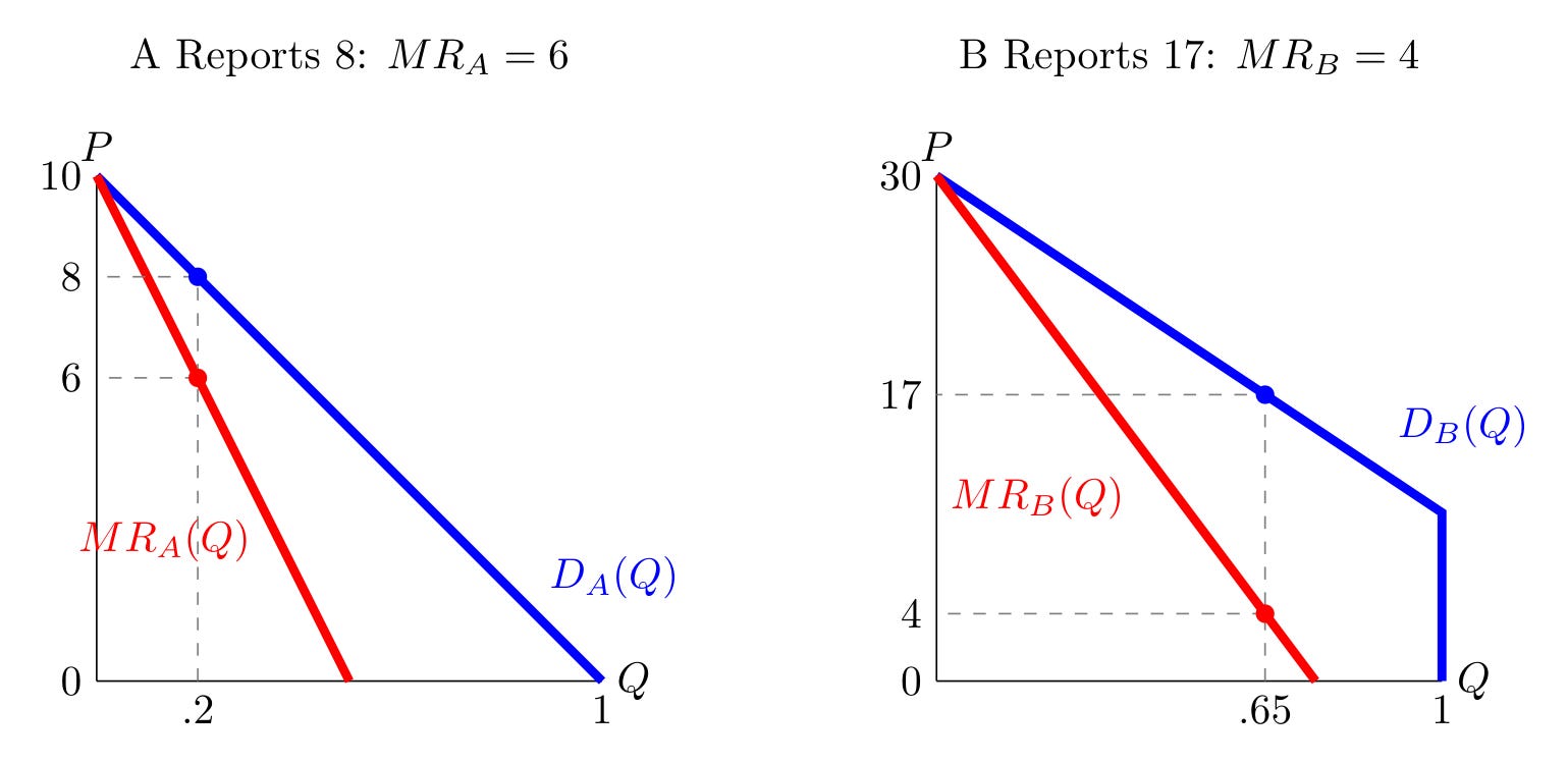
Now let’s let the two bidders differ. Again, I’m gonna follow Bulow and Roberts’ example, so you can check the numbers. Suppose bidder B’s value is uniform between 10 and 30, so B always values the object more than A possibly could. We can do the same thing and draw their marginal revenue curve.
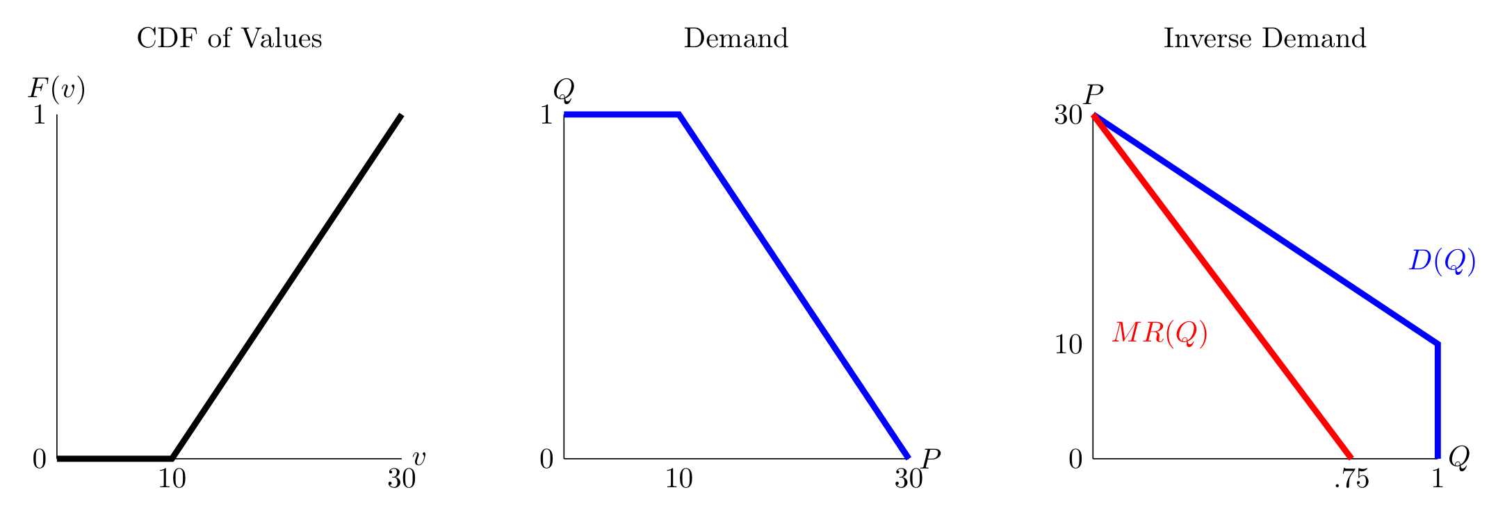
From here, we are able to calculate the reserve price for each market if they were separate: $5 for A and $15 for B, where each marginal revenue curve hits zero.
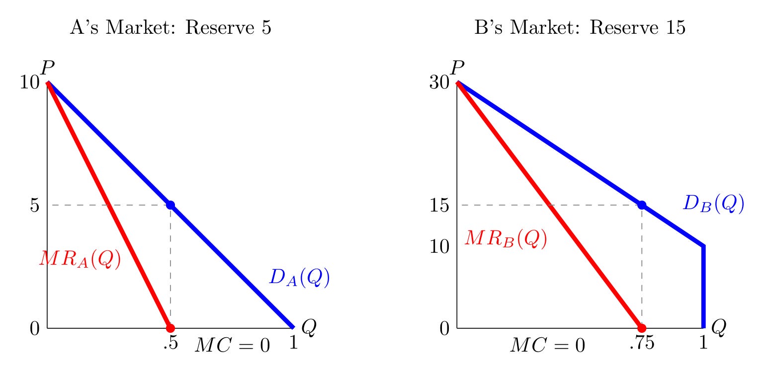
In the price theory, monopoly translation, we can think of each bidder as a separate market. Adding B doesn’t change A’s demand, does not make it more elastic, or change the marginal revenue curve. This competition doesn’t enter through that margin.
Competition instead operates through a capacity constraint. The seller only has one unit. Since we have one unit, the marginal cost is zero up to one and then infinite above that. This jump didn’t matter with one buyer but it does show up with two.
Suppose both bidders bid above their reserves, so the seller cannot serve both, and the marginal cost of the unit in A’s market is no longer zero. The marginal cost (opportunity cost) is what the seller gives up by not selling to B. What she would have collected from B is, on average, B’s marginal revenue. So the marginal cost of the unit in A’s market is B’s marginal revenue at B’s bid.
Selling to the low bidder
So who gets the good? Suppose A truthfully reports a value of $8 and B reports $17.
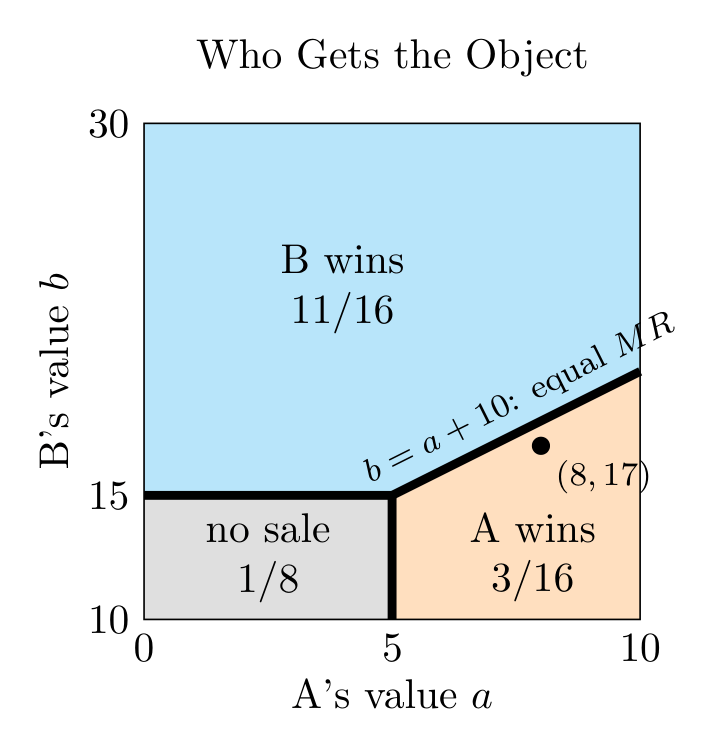
We can go back to their marginal revenue curves and see that the MR for A is 6 and for B is 4. So “on the margin” giving the good to A is more valuable than it is to give to B. We should have a rule that gives the good to the low value in this case. We can keep going and find the boundary at which these MR curves are the same to find the rule.
Set the two marginal revenues equal. A’s is 2a − 10 and B’s is 2b − 30, so they match when a = b − 10.
This turns into the following auction. To determine who wins, subtract $10 from every bid B makes, then run an ordinary second-price auction with a $5 floor. A pays the larger of $5 and b-10, B pays the larger of $15 and a+10.
At $4 and $12, neither bidder is above each’s floor, and the object stays with the seller. At $8 and $17, A clears his floor, beats B’s adjusted bid of $7, and pays $7
Real auctioneers already use both instruments, floors and handicaps, usually for other reasons. Bidding credits for small firms in the FCC’s spectrum auctions are a handicap, and Ian Ayres and Peter Cramton argued they raised the government’s revenue.
As Bulow and Roberts point out, this is just standard optimization, so we can apply this to much more complicated problems. The general rule is “allocate units to the buyers with the highest marginal revenues, by choosing prices to equate the marginal revenues of the lowest-valued buyers actually supplied in each market.”
That’s really all any of this is, whether a fixed price or an auction. People optimize, and adjust. Everything is price theory, if you hadn’t figured that out from this newsletter.
A fun read, even if a lot of this went over my head. The transition from standard monopoly output restriction to auction handicaps actually made sense, though I might need to re-read the part about B's marginal revenue a second time...