Will AI Prove Piketty Right?

What the basics of growth theory say

Philip Trammell and Dwarkesh Patel wrote a fun essay arguing that while Piketty was wrong about the past, AI will make him right about the future. They make two claims I want to address.

1. Labor’s share of income will go to zero.

2. Given that, a global progressive capital tax is “essentially the only way to prevent inequality from growing extreme.”

But reading through the essay (and follow-up discourse), I kept losing track of different parts of the argument. There’s a lot happening in these big, world altering scenarios: how easily machines can replace workers, how fast equipment wears out, differences in investment returns, who actually pays taxes, international coordination.

So instead, as is my wont, let me slow down and revisit supply and demand. In this case, supply and demand for capital. I start with a baseline growth model and ask: which assumptions need to hold for their conclusions to follow?

In particular, their analysis jumps to an extreme endpoint (an economy where labor contributes nothing). Séb Krier has a new piece that reaches basically the same conclusion, that they are looking at a knife-edge.

Getting labor’s share all the way to zero—not from 60% to 30% but to basically zero—requires one of two conditions:

One option is that capital and labor are perfect substitutes. Not just easy to substitute but perfectly interchangeable. This means there’s not a single task in the entire economy where humans have a comparative advantage. Labor becomes worthless regardless of how much capital exists, so its share goes to zero. I touch on this briefly.

The other option—and the focus of their piece through its connection to Piketty—is that capital accumulates without bound faster than labor. Workers still earn something per hour, but capital income grows so large that it dwarfs labor income.

For this to happen, we also need an extreme (from my perspective) assumption. It’s not enough for capital to become more substitutable with labor. For capital accumulation to obliterate labor share, the return on capital must always exceed depreciation plus what savers require to delay consumption, not just now or during a transition, but at every level of capital accumulation, forever. That is a problem if there are ever diminishing returns (say you need land).

Even if there are no land/labor/energy/anything constraints, a different problem arises. The same technological progress that makes substitution easy also makes last year’s AI obsolete. Fast progress raises depreciation through obsolescence. Your GPU doesn’t depreciate only because circuits break. Instead, it depreciates because next year’s model renders it less valuable. And investors have to be rewarded for that loss of value.

Economics is about the process of markets, how they adapt and change prices. The zero-labor endpoint is a knife-edge. Getting there requires passing through regions where standard economic principles apply and where multiple margins adjust simultaneously.

In those regions where labor still plays a role, I don’t think their policy conclusions achieve their ends. Capital taxation hurts workers. If you start with the world as it is today (with capital and labor both contributing) and think about the possible path to a world with zero labor share, their policy proposal to tax capital will only hurt workers. The features of AI they highlight are exactly the features that make capital taxes horrible for workers.

Especially as someone who works on policy and sees knife-edge ideas trickle into policy discourse as if it’s the real world, I want to keep us in that world, while I’m glad others are thinking about other futures.

[I’ve tried to make this as jargon-free as possible. All math is relegated to the footnotes along the way. It should look almost like an appendix at the bottom for people who are interested in the math.]

How the Economy Divides Its Output

We have tools to think through this. Supply and demand. In particular, I want to think about the supply and demand for capital. Since we are trying to understand how we get to a world with zero labor share, we don’t want to assume that. We want to derive whether it’s plausible.

Start with the basics. Total economic output gets divided between workers (as wages) and capital owners (as returns on their investments). These two shares add up to 100%; the whole pie gets divided between workers and capital owners.¹ To simplify things, this is how I’m going to think about inequality. I think that’s a big assumption that I’d like to drop but their piece is heavily framed around the share. And I’ve already written about wage inequality, although as Philip and Dwarkesh point out, capital inequality could be a big deal.

Production today (maybe not at the singularity but today) uses capital and labor. How do firms choose what combination? As always, it depends on prices. When the relative price of labor (wages) rises compared to the cost of renting equipment, firms substitute toward equipment and away from workers. They switch to using more machines and fewer people to produce any amount of output.

The key technological question is how responsive is this substitution? When relative prices change, how much do relative quantities change? If wages rise 10% relative to equipment costs, and firms respond by using 20% more equipment relative to labor, firms are very responsive. High responsiveness means firms aggressively substitute toward whichever factor got cheaper. Low responsiveness means firms are stuck with roughly fixed proportions regardless of prices.

As Philip and Dwarkesh point out, this responsiveness determines how income shares change when the economy accumulates more capital. Most empirical estimates find that firms don’t substitute very easily. The “elasticity of substitution” between capital and labor is well below one, which is below what is needed for the Piketty capital accumulation spiral.²

Raval 2019

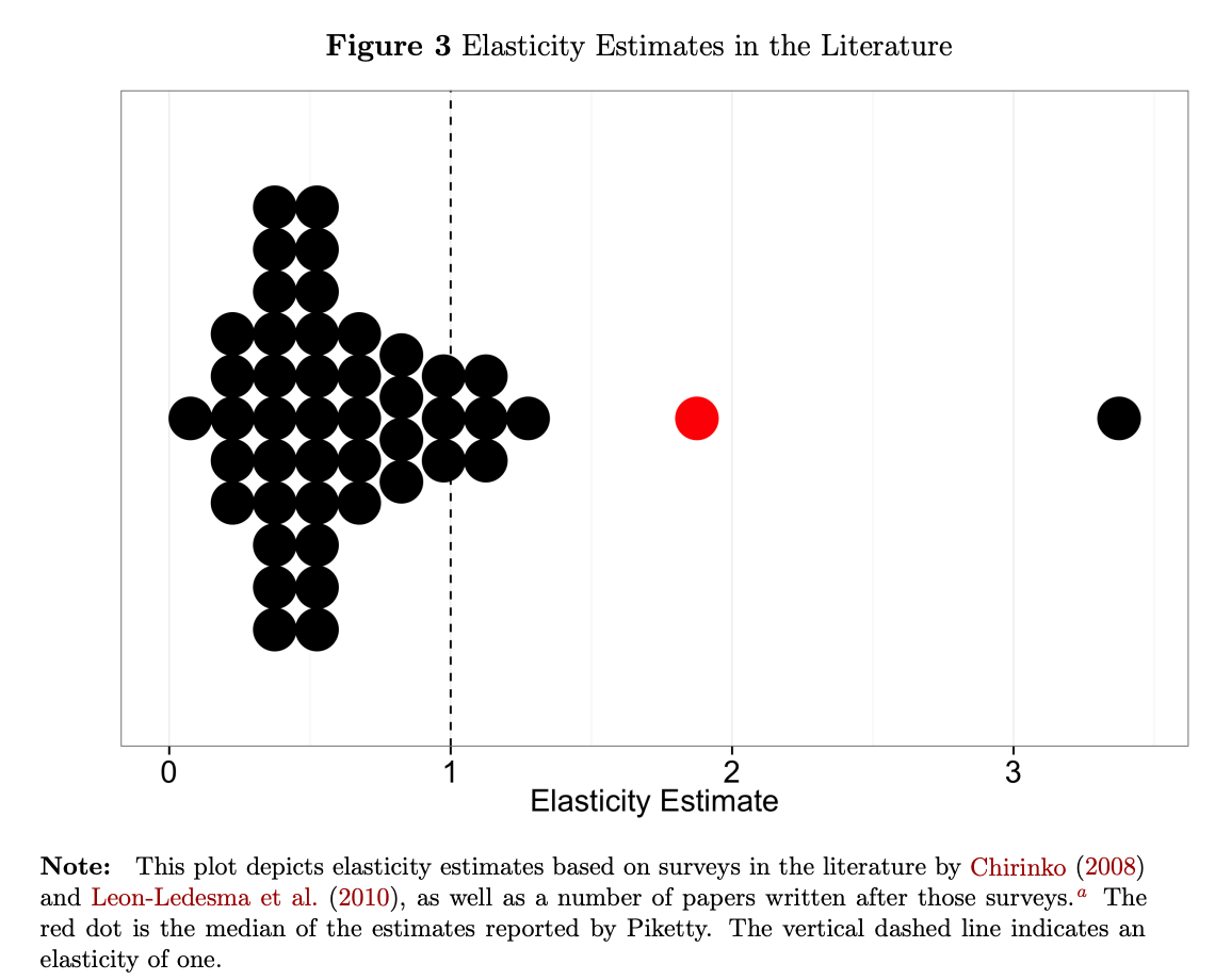
That’s why so many economists pushed back on Piketty’s original argument: capital accumulation has been self-correcting. As societies accumulated more capital, returns fell fast enough that capital’s share of income didn’t explode. This newsletter isn’t a piece about Piketty, but this is the background context.

Trammell and Patel argue AI changes this. When firms substitute easily between capital and labor, adding more capital doesn’t bid down returns as fast as the quantity increases. Capital’s slice of the pie grows. Even if substitution was hard historically, it will become easy once robots can do enough tasks that workers do. I find this plausible.

But how far does this take us? So far this is all technological. Where are the markets? Where is supply and demand?

Supply and Demand for Capital

I’m going to hold the number of workers fixed. This rules out some things people care about in this discourse like workers starving, but as we will see workers don’t starve so that doesn’t really matter in this model. So I can think of everything in per worker terms. How much capital per worker?

Start with demand. In the basic model firms rent capital; they don’t own it. Why do firms demand capital? It helps them produce output that they get paid for. The return they’re willing to pay depends on how much that capital adds to output.

When capital is scarce, firms bid aggressively for it. The return is high. As capital becomes abundant, the standard assumption is that each additional machine adds less value. That’s what we call diminishing returns. The return firms will pay falls as the supply of capital rises.

This gives a downward-sloping demand curve. More capital, lower returns.

Remember that we are always talking ultimately about consumer value. There is decreasing demand for capital because the VALUE that capital generates for the firm is falling. It could be that the capital is just as physically productive, but consumers are willing to pay less for the trillionth semiconductor produced. I think this is crucial point as we start thinking about the slope. But we will get to that in a minute.

Now consider supply. Where does capital come from? Capital comes from investment. Investment comes because people save instead of consuming. They’re willing to do this if the return compensates them for waiting.

The standard assumption (and nothing in the AI story changes this) is that savers require a minimum return. Below that threshold, they’d rather consume today. Above it, they’ll supply as much capital as the economy wants.

This threshold has two components. One is patience: how much return do savers need to delay consumption? Call it 3-5% per year. The other is depreciation: capital wears out, so savers need to earn enough to replace what’s lost before they see any real return. We will spend a chunk of time on that later.

I’m going to assume the supply of capital is upward sloping for now. The first dollar saved requires a lower return than the millionth. I’ll discuss later how this could be upward sloping, downward sloping, or flat, and what drives each case.

To find the capital stock that exists in equilibrium, we need to understand where supply and demand intersect. It doesn’t matter if (I said there’d be no math. I didn’t say no graphs.)

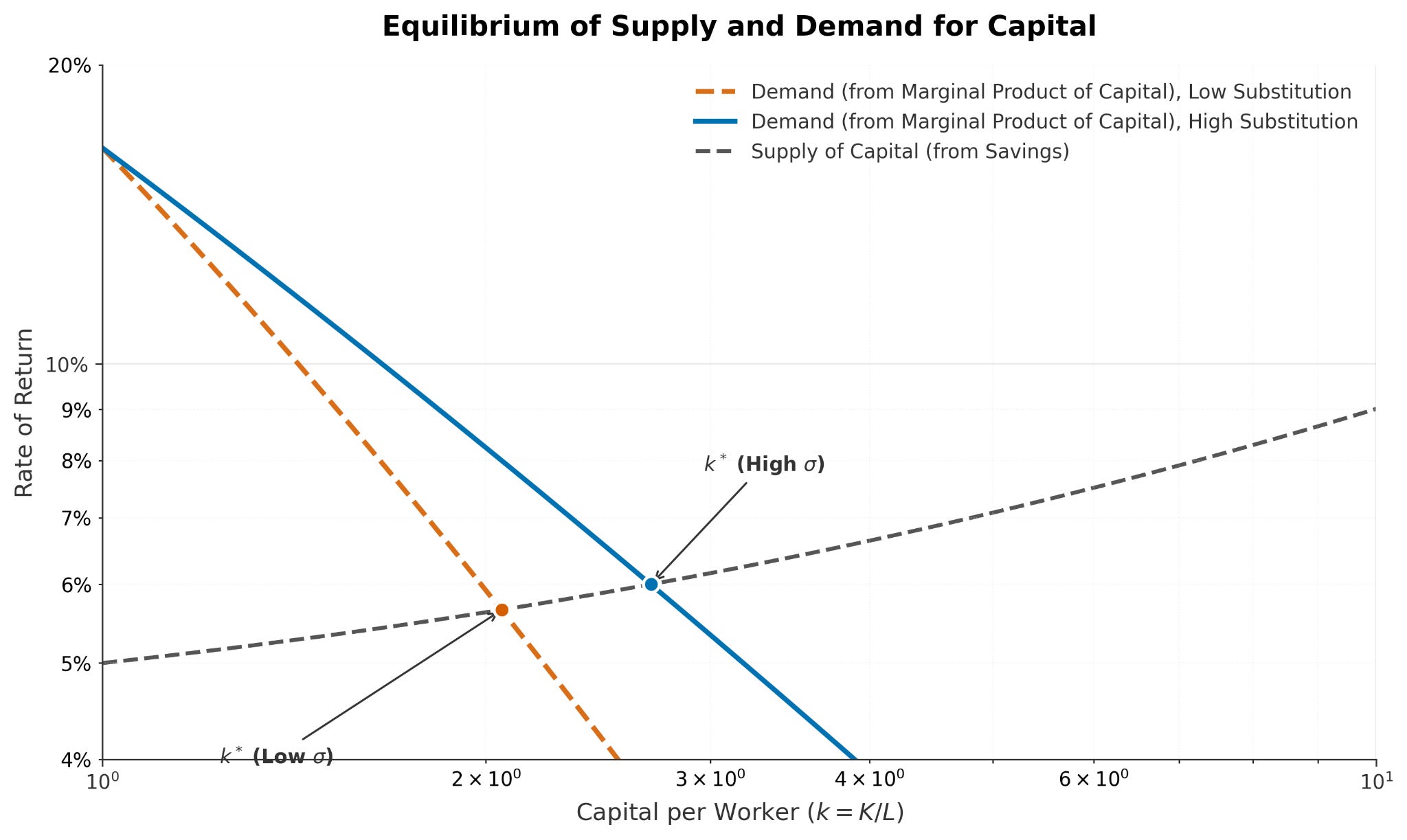
The horizontal axis is the capital stock. The vertical axis is the return on capital.

The demand curve slopes downward; more capital means lower returns. How steeply it slopes depends on a few things, but one that Trammell and Patel focus on and that matters for this discussion is how easily capital substitutes for labor.

If capital and labor are easily substituted, then diminishing returns don’t bite as hard and the demand curve is flatter. That means we will end up with more capital. But if we are still in the elasticity less than 1 world, the demand curve goes toward zero, so will cross the supply curve.

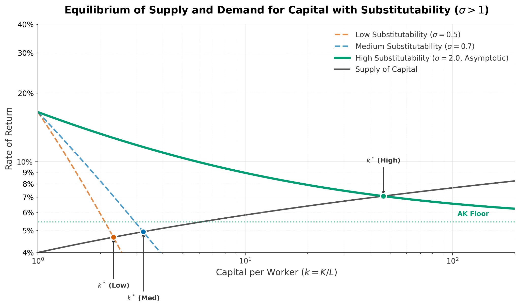
If, however, we are in the world with even easier substitutability (elasticity of substitution greater than 1), then the demand curve will not go to zero but go to some other positive return. No matter how much capital we accumulate, there is still finite value being generated. Remember this is all in value terms.

For now, the supply curve is upward sloping, so it will intersect the demand curve at some point, even in the Piketty world.

Where these curves cross determines how much capital the economy accumulates.

Rising vs. Going to 100%

I’m glossing over a bit by jumping to that equilibrium amount of capital, k*. After all, we want to take the process seriously. We might start below the equilibrium (more properly, steady state) capital and build toward the steady state. That will make more sense when we think about building a capital stock and the role of depreciation below.

It’s important to make clear that capital share rising is not the same as capital share going to 100%. The first requires fewer assumptions. The second requires more.

Claim 1: Capital share rises as capital grows relative to labor (when substitution is easy).

When capital and labor substitute easily, adding capital doesn’t bid down returns as fast as the quantity increases. Capital’s slice of the pie grows, as you’re moving to the steady state. If AI makes substitution easy, capital accumulation raises the capital share instead of being self-correcting. I find this plausible for some range. Absolutely.

But notice: this tells us the direction of change, not the destination. Capital share could rise from 30% to 40% to 70% and then slows down and reach some steady state. That’s a tranformative change but it’s very different from reaching 100%.

Claim 2: Capital share approaches 100%.

In this case, labor becomes negligible. For this to happen, either labor becomes worthless or labor stays somewhat valuable and capital grows without bound.

For labor to be worthless, the elasticity of substitution has to be infinite, not just high (above 1). There’s a big gap between 1 and infinity, even when AI is counting.

Remember this is a model of the whole economy, so that would mean there’s not a single thing produced that humans have a comparative advantage. This would also mean the labor share goes to zero even if output overall isn’t growing.

The other possibility for 100% capital share is that workers still have some pay but capital accumulates and outstrips labor income. That’s the Piketty lens. And not just that, but for capital share to reach 100% capital has to grow without bound. Since this would be the more standard way to generate economic growth (and what I assume will happen under any reasonable model of AI), we should examine how plausible that is.

When does capital grow without bound? Only if the demand curve is always above the supply curve. To see when that happens, we need to be more careful about the shapes.

Where Does Capital Come From?

I’ve glossed over a distinction between investment and capital. Savers invest. That investment possibly accumulates to determine that capital stock.

I say possibly because capital involves depreciation. Every period, a fraction of your machines break down, become obsolete, or wear out. This is depreciation. You need to invest just to stay in place by replacing what’s lost before you can grow.³ The bigger your capital stock, the more you lose to wear and tear each period.

Think of it as a leaky bucket. You’re pouring water in (savings and investment) while water leaks out (depreciation). The leak is proportional to how full the bucket is. A small bucket loses a little water. A big bucket loses a lot. Eventually you reach a level where the water pouring in exactly equals the water leaking out. That’s the steady state.

When we talk about capital’s marginal product, we mean the net return after accounting for depreciation. (We could also flip it around and think about the saver getting a net return). A machine might add $100 to output, but if $10 of that value gets eaten by wear and tear, the net marginal product is $90. Depreciation isn’t a choice or a tax; it’s a physical fact that happens whether you like it or not. Gamma rays hit your semiconductor and mess something up.

This matters because for capital to grow without bound, the net marginal product must stay above what savers require.⁴ Savers have a patience threshold; they’d rather consume today unless compensated enough to wait. Let’s put that at 3-5% per year. If the net return falls below that threshold, they stop accumulating and consume instead.

When does capital grow without bound?

Only if the demand curve NEVER crosses the supply curve. Only if returns stay above the hurdle rate forever, no matter how much capital accumulates. That requires understanding whether the demand curve ever dips below the flat supply curve.

What Determines Savings, aka the Supply Curve of Capital?

Where does the savings rate come from? Households decide between consuming today versus saving for tomorrow.

A household values consumption in both periods. Patience determines how much they discount future consumption. If a household values a dollar of consumption next year at 95 cents today, they’re fairly patient.

If the household saves a dollar today, it earns a net return from the productivity of capital after depreciation has already taken its cut. The household trades off happiness from consuming today against happiness from the larger consumption tomorrow.

In steady state, consumption is constant over time. This pins down the required net return: it must equal the rate of impatience.⁵ Households will supply any amount of capital as long as the net return meets this threshold. Below this rate, they consume instead of saving.

This makes the supply curve flat at the rate of impatience.

Why is the supply curve flat? Two assumptions drive this result, both plausible for thinking about long-run capital accumulation.

The first is that the ability to turn dollars into capital units doesn’t change. A unit of output not consumed becomes a unit of capital; the transformation rate stays constant as you scale up investment. If instead producing investment goods had rising marginal costs—if the tenth billion dollars of investment were harder to create than the first—then the supply curve would slope upward. But with a single consumption-investment good, the trade-off between consuming today and investing for tomorrow stays fixed in the steady state.

Second, the rate of impatience doesn’t shift with wealth.. This means that as capital accumulates and households get richer, they don’t suddenly become more patient and accept lower returns, or vice versa.

Remember this is forever. We are wondering what happens out at the far right. It’s not just whether people will get more or less patient from today but whether impatience eventually stabilizes.

Neither assumption is a deep truth about the world. Both could fail. If producing investment goods has rising marginal cost and you need increasingly expensive inputs as you scale up production, then capital supply slopes up instead of staying flat. If wealthy people become more patient (the rate of time preference falls with wealth), then supply could even slope down. Wealthy households would accept lower returns, which, as we will see, would actually make capital taxation even worse for workers.

But the flat supply curve is a reasonable benchmark for long-run analysis. The supply curve sits flat at the rate of impatience, again maybe 3-5% per year. Remember, this is the net return savers require, after depreciation has already been accounted for in what capital actually delivers.

Paths to Zero Labor Share

The zero-labor-share outcome can happen two ways. Each requires different conditions.

Path 1: Labor becomes worthless.

I went over this quickly, but it’s worth mentioning again. This happens if capital and labor are perfect substitutes. Not just easy to substitute—perfectly interchangeable. Not just elasticity above one—infinity.

In this world, if a robot can do a task 1% cheaper than a human, firms switch entirely to robots. No mixing. No comparative advantage for humans in anything. Labor’s marginal product falls to zero regardless of how much capital exists.

Path 2: Labor stays somewhat valuable, but capital grows without bound.

This is the Piketty-style path. Workers still earn something per hour, but capital accumulates so fast that capital income dwarfs labor income. The ratio of capital to labor goes to infinity.

This requires the elasticity of substitution to exceed one (which we don’t see in the data), but it doesn’t need to be infinite. Capital and labor can still complement each other somewhat. The question is whether capital keeps accumulating forever.

For that to happen, the demand curve for capital must NEVER cross the supply curve. Returns on capital must stay above the hurdle rate (depreciation plus impatience) no matter how much capital exists. If returns eventually fall below that threshold, accumulation stops at some finite level. Capital share might be high—60%, 70%, 80%—but not 100%.

Three Scenarios

I’m going to again not worry about the perfect substitution case.

This gives us three paths for the capital share, not two:

Scenario A: Historical. Capital and labor complement each other. The demand curve slopes steeply from diminishing returns, crosses the supply curve, and we get a finite steady state. Capital share is stable around 30-40%. This is the world Piketty’s critics described.

Scenario B: Transition. Capital and labor substitute easily. The demand curve is flatter. Capital share rises as capital grows relative to labor. But depreciation is high enough that the curves still cross at a finite point. Capital share might reach 50%, 60%, even 70%, but not 100%. Labor still matters. Standard economics still applies.

Scenario C: Zero-labor endpoint. The demand curve stays above the supply curve and depreciation forever. Capital grows without bound. Labor share falls toward zero. This is the Trammell-Patel world.

The essay jumps from “substitution will become easy” directly to Scenario C. But Scenario B is a logical possibility they don’t address. And Scenario B is where we’d spend a lot of time on the transition path, even if we’re eventually heading toward C.

What Does “Robots Building Robots” Mean?

This phrase appears throughout discussions of AI and capital. But what does it actually mean for the model’s parameters?

The phrase could involve several distinct mechanisms. All four imply a higher equilibrium capital stock. All four make it more likely the demand and supply curves never cross.

Interpretation 1: Easier substitution between capital and labor.

Robots building robots could mean capital brings its own complementary inputs. Historically, adding capital required proportionally more labor to maintain, operate, and coordinate the machines. Every new machine needed workers to run it. If AI capital maintains itself, the “not enough hands” constraint weakens. Diminishing returns slow. This is about production technology.

This is the interpretation the essay emphasizes. This flattens the demand curve. Returns stay higher as capital accumulates.

Interpretation 2: Weaker diminishing returns overall.

Even holding labor fixed, capital might face weaker diminishing returns if it doesn’t hit other bottlenecks. Traditional capital runs into scarce energy, rare materials, specialized components. If robots can substitute for these inputs too—mining their own materials, generating their own power, fabricating their own parts—then returns don’t fall as fast.

This also flattens the demand curve, for reasons beyond labor substitution, in a fuller model with land and energy.

Interpretation 3: More efficient investment.

Robots building robots could mean capital is cheaper to produce and replace. Installation costs fall. Adjustment frictions disappear. Replication accelerates.⁶

This lowers and possibly flattens the supply curve. If replacing depreciated capital costs less, savers don’t need as high a return to keep accumulating. The hurdle rate falls.

This is what I think Trammell and Patel mean with their “self-replicating robot factories”—capital that can reproduce itself without hitting bottlenecks. Each dollar of saving deploys more effective capital. The wedge between “dollars saved” and “machines working” shrinks.

Interpretation 4: More mobile capital.

Robots building robots could mean capital is easier to relocate. If robots can be shipped anywhere, built anywhere, operated remotely, capital flows freely to wherever returns are highest.

This flattens the supply curve. Capital faces fewer local bottlenecks, so any profitable opportunity gets funded.

Each interpretation works through a different mechanism: two flatten demand, two lower or flatten supply. But they all push in the same direction: more capital in equilibrium, and a better chance the curves never cross.

This is the interpretation the essay emphasizes. Fair enough. But notice: for unbounded growth, you need these effects to be strong enough that the curves never cross. That’s a quantitative claim, not just a qualitative one.

Will AI Depreciate Faster? Depreciation Question

Fast technological progress is what makes substitution easier. AI improves and replaces more labor. But fast progress also means last year’s AI becomes obsolete. Think about how dated AI models feel from a few months ago, let alone years.

The same force that flattens the demand curve raises the hurdle rate.

Think about what it costs to own a machine for a year. An investor who buys equipment today and rents it out must earn enough to cover three distinct costs:

There’s an opportunity cost. The money tied up in the machine could have earned interest elsewhere. If you spent $100,000 on a robot, that’s $100,000 not sitting in a bond earning 5%. Remember, we are already accounting for this through household impatience.

There’s physical wear. The machine breaks down, parts wear out, maintenance accumulates. A truck’s engine has finite miles. A robot arm’s joints degrade.

There’s obsolescence. The machine becomes outdated. Next year’s model is faster, cheaper, more capable. Your equipment still works, but nobody wants to rent last year’s technology when this year’s does the job better.

This third component is the killer for the “robots building robots” story.

Your GPU doesn’t depreciate just because circuits break. It depreciates because next year’s model renders it worthless. Physical decay might be 5% per year. But if last year’s AI model is uncompetitive against this year’s, obsolescence could add another 20-30%. Value depreciation of 30% per year is plausible for cutting-edge AI hardware.⁷

Here’s the tension: fast progress flattens the demand curve but also raises the supply curve. Whether the curves cross depends on which effect dominates.

If depreciation is 30% and impatience is 3%, the hurdle is 33%. The limiting productivity of capital must exceed 33% for capital to grow without bound. That’s a high bar.

And it’s not enough to clear that bar once. You have to clear it forever.

For capital to grow without bound, the return on the next machine must exceed the hurdle rate no matter how much capital already exists. Not just when capital is scarce and returns are high. Not just during a transition period. At every point along the path, and out to infinity.

If there’s any capital stock at which the marginal return dips below depreciation plus impatience (even far in the future, even at capital levels we can barely imagine) accumulation stops there. The curves cross. You get a finite steady state. Maybe a very high one, with capital share at 70% or 80%. But finite.

The zero-labor-share outcome requires that capital always generates at least a 30% return and the lines never cross.

Maybe that’s plausible in a different model, but if we are taking the benchmark economic growth model off the shelf, it’s a lot to ask.

Should we tax capital?

Suppose they win the race. Suppose AI does make substitution so easy, and depreciation stays low enough, that capital grows without bound and labor’s share falls toward zero. Grant them the inequality story.

What about the decades before labor share goes to zero? (Grant me it won’t happen for two decades). Does the policy conclusion follow?

Their answer is a global progressive capital tax which is ”essentially the only way to prevent inequality from growing extreme.” If capital owners are capturing an ever-larger share of income, tax that income and redistribute it.

The logic seems straightforward. But it runs into a problem: the same features that make capital accumulation explosive are exactly the features that make capital taxation ineffective.

The essay focuses on how easily capital substitutes for labor in production. Thousands of words on this parameter. But who bears a tax depends on a different question: how responsive is capital supply to changes in the required return?

These are separate concepts doing separate work.

Substitutability in production measures how much the return on capital falls as you add more capital. It’s the slope of the demand curve. High substitutability means a flat demand curve. You can add a lot of capital before returns fall much.

Responsiveness of capital supply measures how much the capital stock changes when the required return changes. If savers demand a fixed after-tax return regardless of how much capital exists, supply is perfectly responsive. The supply curve is flat. Any return above that level brings forth unlimited capital; any return below it causes capital to disappear.

Who bears a tax depends on which factor can escape. Same tax, same production technology, same substitutability, but different burden depending on what can move.

For the AI scenario Trammell and Patel describe, responsive capital supply is the relevant case. They’re thinking about long-run dynamics where capital accumulates over generations. And their own language supports it. They describe “self-replicating robot factories” that “can easily go anywhere.”

This points toward increasingly elastic supply, maybe even perfectly elastic like the benchmark model.

So what happens when you tax capital with elastic supply?

Households won’t supply capital unless the after-tax return equals their required return. They have a patience level. If returns fall below it, they consume instead of saving. In the long run, accumulation adjusts until returns exactly meet their requirement.

This means if you impose a tax, the pre-tax return must rise to compensate. Capital owners end up with the same after-tax return as before. They’ve escaped the tax.

But the pre-tax return is what firms pay. If firms must pay higher returns to attract capital, something else has to give. That something is wages.

This is a standard result: with responsive capital supply, a capital income tax lowers wages. Capital escapes. Labor pays.

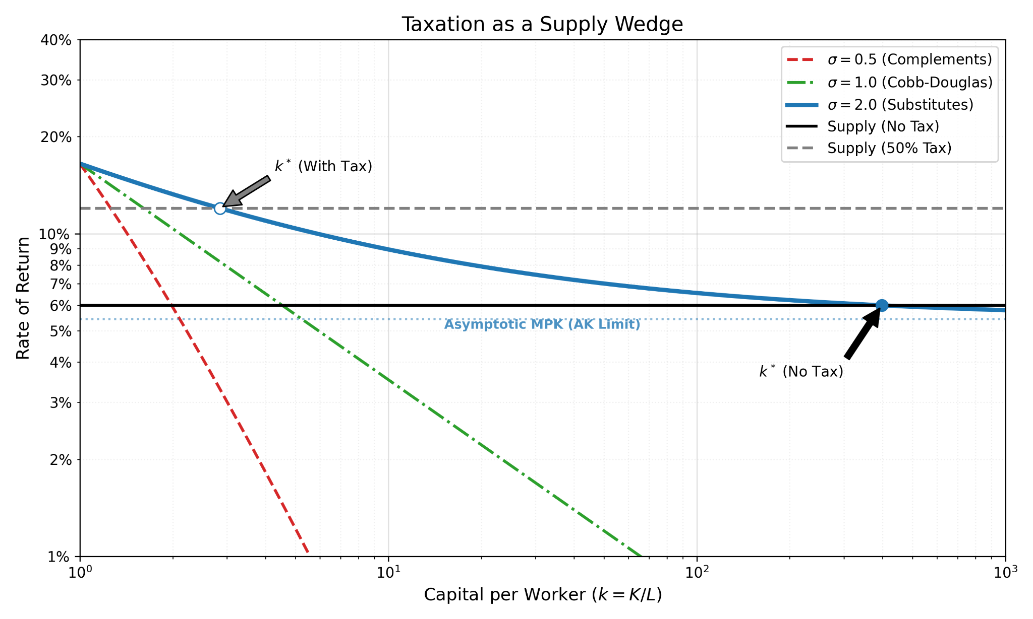
What role does substitutability play? It determines how severely the economy contracts. Yes, high substitutability means firms can aggressively expand capital

It also means that firms aggressively shed capital when they are taxed. The capital stock shrinks MORE!. Output falls more. Workers lose more.⁸

High substitutability means workers are easily replaced by machines. That’s the inequality story. But it also means firms respond aggressively to any increase in capital costs. A flatter demand curve means capital flees faster when taxed, and labor bears a heavier burden through lost wages.

The features Trammell and Patel invoke for their inequality story are the same features that undermine their policy story.

The Policy Tension

For capital share to approach 100%, Trammell and Patel need capital to accumulate aggressively. They describe robots that replicate, factories that relocate, capital that flows freely to wherever returns are highest. Elastic supply is doing work for their inequality story.

For capital taxation to help workers, they need the tax burden to stick to capital owners. This requires inelastic supply. If capital can escape—by flowing elsewhere, by not being accumulated, by being consumed instead of saved—then taxing it shrinks the economy and wages fall.

These cannot both be true. The features that make capital accumulation explosive are the same features that make capital taxation ineffective.

The authors recognize this partially when they call for international coordination. If all jurisdictions tax capital equally, there’s nowhere to flee. But this only solves the mobility problem. It doesn’t solve the accumulation problem.

Even with perfect global coordination, savers can still escape the tax by not saving. If the after-tax return falls below their patience threshold, they consume instead of accumulating. It’s not that capital doesn’t flow to another country. It simply doesn’t get built.

The Path to Singularity Matters

The essay treats easy substitution as if it immediately implies an economy where labor contributes nothing. But easy substitution is a local condition about how factor shares respond to capital growth. Getting to zero labor requires passing through a transition where labor still matters, where multiple margins adjust simultaneously, and where standard economics applies.

In Scenario B—where substitution is easy but we don’t reach the zero-labor endpoint—standard policy tools still work. Labor income still exists to tax. Human capital investment still has returns. Wage subsidies still have a target. The economy looks different from today, more capital-intensive, but it’s not a different planet.

In Scenario C—their world—labor income approaches zero, and “tax capital” becomes the only option by process of elimination. (At least, according to Trammell and Patel. As Basil Halperin points out, we can still tax consumption or a fixed factor like land). But taxing capital in a world of responsive capital supply doesn’t help workers. The features that get you to Scenario C are the same features that make capital taxation fail.

I don’t know the answer to most of the predictive questions here. How easily will capital substitute for labor? How much will consumers switch away from human services? How fast will depreciation rise? How mobile will capital actually be? How patient are the rich? I know estimates from today and they are far off from the assumptions.

But the baseline model helps me see what’s at stake. The jump from “substitution might become easy” to “global capital taxation is the only way” requires being on the right side of multiple separate conditions simultaneously. Some plausible, some unknown, some in tension with each other.

Trammell and Patel ask a genuinely important question: what happens to factor shares and inequality if AI can do everything humans can do?

I have no idea. But I’m confident that the path matters and economics can help us think through things. The endpoint where labor contributes nothing is a limiting case. Getting there (if we ever do) involves passing through regions where standard economic principles apply and where multiple margins adjust. That’s where we actually live, and that’s where policy has to operate.

1. Output Y comes from capital K and labor L. Factor prices equal marginal products: wages W and rental rate R. Define income shares:

\(s_L = \frac{WL}{Y}, \quad s_K = \frac{RK}{Y}\)

Cost minimization requires the marginal rate of technical substitution to equal the factor price ratio:

\(\frac{F_L}{F_K} = \frac{W}{R}\)

2. The elasticity of substitution σ\sigma σ measures responsiveness:

\(\sigma = \frac{\%\text{ change in } K/L}{\%\text{ change in } W/R}\)

This gives a relationship between price and quantity changes:

\(\Delta W - \Delta R = \frac{1}{\sigma}(\Delta K - \Delta L)\)

3. Capital accumulation follows:

\(\dot{K} = sY - \delta K\)

Savings sY adds to the capital stock. Depreciation δK subtracts. Steady state occurs where these balance: sY=δK. For unbounded growth with easy substitution, sA>δ where A is the limiting productivity of capital.

4. Since the net return is r=MPK−δr, the condition for accumulation becomes:

\(MPK > \delta + \rho\)

With easy substitution, the condition for unbounded growth:

\(\bar{A} > \delta + \rho\)

where Abar is the limiting marginal product of capital.

5. Households maximize utility

\(U(c_0) + \beta U(c_1), \quad {where} \quad \beta = 1/(1+\rho) \)

captures impatience. The optimality condition:

\(\frac{U'(c_0)}{\beta U'(c_1)} = 1 + r\)

In steady state with constant consumption: r=ρ. The net return must equal the rate of time preference.

6. Expand the model with an efficiency parameter η:

\(K_{t+1} = (1 - \delta)K_t + \eta_t I_t, \quad 0 < \eta_t \leq 1$\)

Here I_t​ is resources devoted to investment through foregone consumption. The parameter η​ measures how efficiently investment translates into effective installed capital.

If η=1: one unit invested becomes one unit of effective capital. This is the one-good benchmark where output not consumed becomes capital at a fixed rate.

If η<1: some investment spending gets absorbed by frictions like installation costs, adjustment costs, coordination overhead, learning curves. A dollar of foregone consumption yields less than a dollar of productive capital.

The parameter η acts as a wedge between “resources sacrificed” and “machines working.” When η is low, capital is expensive to build. Savers need higher gross returns to justify investment because each dollar buys less effective capital.

The “robots building robots” story maybe implies η→1: self-replicating capital eliminates installation frictions. Investment translates directly into productive capacity without waste. This lowers the effective cost of capital accumulation, shifting the supply curve down and making unbounded growth more plausible. Notice is it bounded at 1.

7. The rental price of capital R_t reflects what firms must pay to use a machine for one period. From the arbitrage condition (buying capital, renting it out, then selling the depreciated remainder) we get:

\((1+r)P_t = R_t + P_{t+1}(1-\delta)\)

Rearranging

\(R_t = rP_t + \delta P_{t+1} + (P_t - P_{t+1})\)

The rental rate has three components. First, opportunity cost (rPt): the return foregone by tying up funds in this machine rather than lending them out. Second, physical depreciation ($δPt+1$): compensation for wear and tear because parts break, joints degrade, circuits fail. Third, capital losses (P_t - P_t+1): the decline in resale value from one period to the next. This captures obsolescence: next year's model is faster, cheaper, more capable, so this year's model commands a lower price.

8. With a proportional tax τ on capital income and perfectly elastic capital supply the after-tax return is pinned down by savers’ required return. A convenient log-change statement is:

\( \Delta \ln R + \Delta \ln(1-\tau)=0,\)

i.e. if \((1-\tau)\) falls, the pre-tax required return \(R\) must rise. With income shares and (log) growth accounting, one common reduced-form way to express the wage impact is:

\( 0 = s_L \cdot \Delta \ln W + s_K \cdot \Delta \ln R,\)

which implies

\( \Delta \ln W = \frac{s_K}{s_L}\cdot \Delta \ln(1-\tau).\)

Since

\(\Delta \ln(1-\tau)<0\)

A convenient expression for how strongly capital shrinks is

\( \Delta \ln K = \frac{\sigma}{s_L}\cdot \Delta \ln(1-\tau) < 0,\)

so high σ means capital flees more aggressively when taxed.