Will lab-grown beef raise the price of handbags?
On the theory of joint production
You are reading Economic Forces, a free weekly newsletter on economics, especially price theory, without the politics. Economic Forces arrives weekly in the inboxes of 12,000 subscribers. You can support our newsletter by sharing this free post or becoming a paid subscriber:
Recent scientific advances have Chanel and Louis Vuitton execs worried. Actually, I have no idea if that is true. I don’t know anyone at any fashion company. But they should be thinking about it!
Namely, what happens as lab-grown beef falls in price and becomes a closer substitute for conventional beef? Fewer beef burgers will mean fewer cattle raised for meat, tightening the supply of hides available for leather.
The key to understanding the connections is price theory. Of course. More specifically, we need to understand a simple extension of supply and demand known as “joint supply” or “joint production.”
Theory of Joint Production
Where most economic models simplify to one product coming out of the production process, joint output systems are multidimensional by nature. Different goods might share biological building blocks, manufacturing equipment, or skill sets. Whatever the tie, changes in demand for one output reverberate through markets and change the availability of the others. As we often say here, markets are connected.
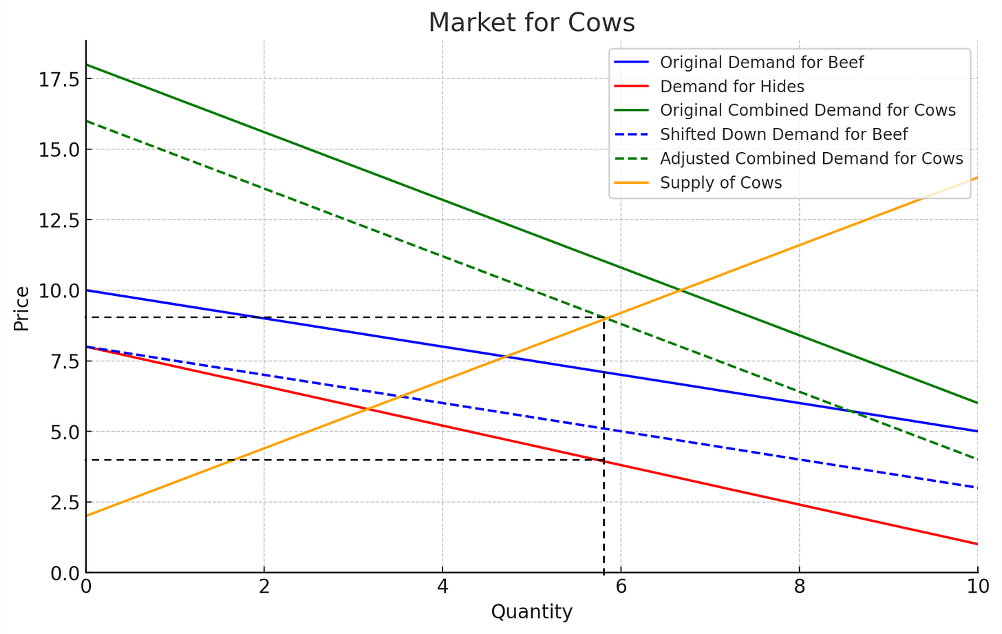
So, how do we model these interconnected markets? There are two parts. First, the willingness to pay (the height of the demand curve) is the vertical sum of the components. If the beef is worth $2 and the hide is worth $1, the joint value of the cow is $3. There are ways to complicate it, but that’s the basic idea. Graphically, if cows are made up of beef and hides in fixed proportions, you stack demand for beef on top of demand from hides to assess total value of the cow. (This “vertical summing” is in contrast to standard models that sum demand horizontally across different consumers for the same good.)
As usual, the equilibrium quantity of cows will be determined by the intersection of the supply of cows. But underneath that, there is a story about beef and hides. The black dashed lines illustrate the equilibrium quantity of cows (over 6), and the corresponding price of beef and hides.
A simplifying assumption above is that goods are produced in completely fixed proportions. More realistically, there is often some flexibility in the ratio of outputs via production choices and tradeoffs. Up to a point, farmers can choose to produce more hides relative to beef. These are complications on the basic model.
Many goods are produced jointly. Moving away from animal examples, oil refining leads to joint outputs of gasoline, heating oil, diesel, and other petroleum products. Wood leads to lumber and shavings. But it’s much more general and includes even things like the production of fancy cars and social status. The value is the “use value” and the “social value.” My favorite example is probably the joint production of knowledge and products that happens in a learning by doing situation.
These jointly-produced goods connect together supply and demand in interesting ways that vary from the standard one-input, one-output model taught in introductory economics.
Lab-Grown Beef and Leather Prices
Now let’s turn to our opening example. As lab-grown beef’s quality improves, that will likely decrease the demand for normal beef. How do the other markets play out?
The basic idea is that less demand for beef reduces the number of cows that are raised. Fewer cows means more expensive hides, leather, and, ultimately, handbags. Once we’ve been explicit about supply and demand, it’s a pretty trivial statement. But that’s usually the case.
To make sure we are mixing up our supply curve with the quantity supplied, let’s draw it out.
Lab-grown beef shifts in the demand for beef to the dashed blue line. That also shifts in the green line, which is a movement along the supply curve and a decrease in quantity supplied. Now, less than six cows are produced, which raises the price of hides on the red line. Done and done.
The topic of joint supply is rarely in modern undergraduate textbooks. McCloskey (1985) is the most recent to have it that I’m aware of.
Again, the idea of joint production shows up again and again. From a pedagogical point of view, the example shows how slight modifications of the standard supply and demand curves can be used to gather insights. It’s just another tool, much like the total supply curve I explained in a previous post that readers have found helpful.
Understanding these interconnections is what price theory is all about. This post just begins to scratch the surface of joint production’s implications. How do substitute technologies affect farmer incentives on managing land between crops holistically? Which outputs share production inputs across the economy, from minerals to manufacturing? And where might we miss key constraints that transmit impacts? Thinking through jointness teaches humility about complexity and not leaning too heavily on narrow, single markets.
In the end, it’s a small tweak to standard analysis but one that better reflects most real world supply relationships. Tracing the threads reveals strange bedfellows — here connecting synthetic food scientists and luxury fashion execs. Joint production will continue to surprise. But surprises beget insight.


People used to eat a lot more lamb and mutton because the demand for wool was much higher before synthetic fabrics.
I think sheep leather became really fashionable for awhile in the 1980s(?) and prices jumped but supply didn't increase that much because joint production.
What an incredibly powerful headline! This is a good point. It happens so often in our increasingly managed economies that there isn’t a comprehensive view of the impact of policy decisions.