No. You can’t compare tariff rates and income tax rates.

John Lott makes a very elementary mistake

A little while back, John Lott had a very confused piece in the New York Post. In it, he made the following claim:

Distortions increase as tax rates do.

Before Trump’s policies, the average US tariff rate stood at just 2.5% — tiny compared to the 43.4% average top personal income tax rate (including federal and state taxes) or the 27.5% average total corporate tax rate.

If we understand a tariff as a tax like any other, higher tariffs could in fact reduce the overall economic burden on American individuals and companies — an outcome that Trump has often touted as his ultimate goal.

This sounds plausible. It sounds like something an economist would say.

But it’s absolutely wrong.

No one corrected him on this. Even economists who pushed back on Lott missed it or ignored it. Don Boudreaux granted “tariffs might well have a role to play as part of the mix of taxes to raise revenue.” David Henderson wrote:

We do know that the deadweight loss, which is the overall loss from the tax minus the gain to the government, is proportional to the square of the tax rate. For example, doubling a tax rate quadruples the deadweight loss. So, it could be true that reducing the top marginal tax rate on income from its current 37 percent to, say, 35 percent, and replacing it with a 5 percent tax on imports could reduce overall deadweight loss.

No. This isn’t possible.

So someone needs to refute this logic outright.

Today’s newsletter has two parts. The first part covers the basic intuition and the second will be the actual math. Putting it in an explicit model will show us the errors and why it’s helpful to be comfortable writing down some math here and there. That’s today’s newsletter. Let’s roll.

The Tax Rate/Deadweight Loss Connection (And Why It Doesn’t Mean What Lott Thinks)

Lott’s claim contains a grain of truth: deadweight loss from taxation increases with the square of the tax rate. Double a tax rate, and you quadruple the deadweight loss. This is a standard result in public finance, and it suggests we should spread our tax burden across many bases rather than concentrate it in one place.

Here’s the intuition. When you impose a small tax, you only kill off marginal transactions—deals that barely made sense in the first place. The buyer was almost indifferent about purchasing, or the worker was almost indifferent about working that extra hour. These marginal transactions don’t create much surplus, so losing them doesn’t cost much.

But as you increase the tax rate, you start killing off transactions with larger and larger surplus. Beyond eliminating the deals that barely made sense, you’re now eliminating deals where both parties really wanted to trade, where there were substantial gains from the exchange. The surplus lost from these inframarginal transactions is much larger.

This is why deadweight loss grows with the square of the tax rate. Double the tax, and you lose transactions that had twice the surplus. The effect multiplies. A 10% tax might eliminate deals that create $1 of surplus each, but a 20% tax eliminates deals worth $1 and deals worth $2. The total loss is 4x, not 2x.

This is the grain of truth in what Lott is getting at. It’s a basic result that people should know.

But Lott pattern-matches from this true principle to a completely invalid conclusion.

Elasticities Matter

That principle compares a fixed market with a fixed demand and supply curve. This relationship only holds within a given tax base. If you want to compare across markets, you need another basic idea from taxation: deadweight loss depends on elasticities.

Elasticities destroy any attempt to compare tax rates across different bases and make Lott’s whole construction nonsense.

Different goods have different elasticities. Some supplies are essentially fixed—you can’t create more of them no matter how high the price goes. Other goods can be produced in unlimited quantities at constant cost. Some demands are highly elastic (people readily substitute to alternatives), while others are inelastic (people need the good regardless of price). These elasticities determine how much distortion a given tax rate creates. The tax rate alone tells you nothing.

More elastic demand or supply curves generate larger deadweight losses. The flipside is the classic Ramsey result: tax less elastic goods more heavily. This assumes the markets aren’t connected, which we’ll address next.

Hilary Hoynes lecture notes

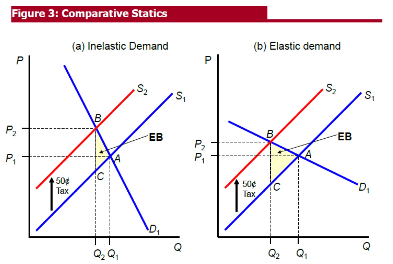
Consider taxing a good with a perfectly inelastic supply—say, land in a specific location. The supply curve is vertical. No matter what price landowners receive, they supply the same amount of land because they can’t create more of it. By definition, there is no deadweight loss. The tax doesn’t change behavior.

What happens when we increase the tax rate on land? The tax raises revenue, but it generates no deadweight loss. Landowners absorb the entire tax through lower prices, but the quantity of land traded doesn’t change. There’s no distortion in the allocation of resources. You could tax land at 100%, and the deadweight loss would still be zero.

This demolishes the idea that you can look at tax rates in isolation. There is no nice connection between tax rate and deadweight loss that transcends the specific good being taxed.

Now compare this to a tariff on imported goods, where supply and demand are both elastic. The tariff creates a wedge between what consumers pay and what producers receive. This wedge distorts both consumption decisions (people buy less than they would otherwise) and production decisions (domestic producers make more than they would in an undistorted market). We get the classic deadweight loss triangle.

The formula that deadweight loss increases with the square of the tax rate applies to both taxes. But it tells us nothing about which tax we should increase. The land tax, even at a 100% rate, might generate zero distortion. The tariff, even at a 2.5% rate, creates real costs. Elasticities matter. You can’t compare tax rates across different bases without accounting for how responsive behavior is to each tax.

Taxes Interact

Lott’s argument has a second problem: tariffs and income taxes don’t operate in isolation.

Suppose people must spend everything they earn; they don’t save. In this case, a 10% income tax is economically identical to an 11.1% consumption tax.

Here’s why. Imagine you earn $100. With a 10% income tax, you keep $90 to spend on consumption. With an 11.1% consumption tax and no income tax, you have $100 to spend, but prices are 11.1% higher. So $100 divided by 1.111 gives you $90 of real consumption. The two taxes create the same wedge between your labor and your consumption.

This equivalence shows you can’t look at the nominal rates and conclude that one tax is lower than the other. If income taxes are at 40% and tariffs are at 2.5%, you can’t say “let’s raise tariffs because they’re so much lower.” You need to compare the actual wedges these taxes create, which depends on how they interact with each other and with people’s economic decisions.

Consider a simple setup. You work for a wage, pay income tax, and face consumption prices that include tariffs. Your budget constraint shows that the income tax and consumption tax compound—they don’t operate independently. The total wedge between your labor and consumption depends on both tax rates together. If the income tax is 40% and there’s no consumption tax, the wedge is 40%. If the income tax is 30% and the consumption tax is 16.666%, the wedge is also 40%. The two combinations are equivalent in terms of distorting your labor supply decision.

In fact, in the case of labor and consumption tax, there’s an easier way to see why you can’t compare: a 100% income tax is equivalent to an INFINITE consumption tax. With a 100% income tax, you keep nothing from your earnings, so you can’t buy any consumption regardless of the price level. With an infinite consumption tax and no income tax, you have earnings but prices are infinitely high, so again you can’t buy any consumption. The two create identical outcomes even though the nominal rates are 100% versus infinity.

This extreme case shows why Lott’s comparison is nonsensical. If we took his logic seriously, we’d conclude that replacing a 100% income tax with “only” a 1,000% consumption tax would reduce distortions because 1,000% is so much smaller than infinity. Obviously this is absurd—both policies would completely shut down the economy. You cannot compare nominal tax rates across different bases and conclude anything about relative distortions. The rates operate on different quantities and compound in different ways.

That’s just a quirk that can be avoided by properly defining tax rates. But in the way we usually talk about them, a 100% income tax is very different from a 100% consumption tax.

The more important point with actual economic content is that we can’t just look at the individual rates and determine which one to raise. Taxes that look small in isolation can create large wedges when layered on top of existing taxes. They compound, affecting workers through the same mechanism.

Imports aren’t consumption taxes

But tariffs are worse than general consumption taxes because they tax only some goods—and imports are a small share of total consumption.

In the US, imports are roughly 10% of consumption. This means tariffs apply to a base that’s ten times smaller than a general consumption tax would. When Lott compares a 2.5% tariff to a 40% income tax, he’s ignoring that these rates apply to completely different denominators.

Think of it this way: if you want to raise $100 from a tax that applies to everyone’s $1,000 of consumption, you need a 10% rate. But if you want to raise that same $100 from a tax that only applies to $100 of imports (10% of consumption), you need a 100% rate. The narrow base means you need a much higher rate to raise equivalent revenue.

This logic applies to any narrow excise tax. By Lott’s reasoning, we should be able to reduce deadweight loss by taxing sugar more on the margin instead of having a broad consumption tax. After all, sugar-specific taxes are lower than payroll tax or income tax rates, right?

But a sugar tax raises revenue from a tiny fraction of consumption. To raise meaningful revenue, you need astronomical rates that create massive distortions in consumption patterns—people completely restructuring their choices because the tax makes sugar prohibitively expensive. It may even be impossible for reasons related to the Laffer curve. The deadweight loss per dollar of revenue raised is much higher than a broad tax, even though the nominal rate might look comparable.

If you think taxing sugar delivers some other benefit (like correcting a health externality), fine. But to raise revenue? It’s strictly worse than a broad consumption tax.

The same logic applies to tariffs versus general consumption taxes or income taxes. Tariffs are excise taxes on imported goods. The narrow base means you need high rates to raise revenue, and those high rates create large distortions.

This gets worse when we account for how tariffs interact with income taxes. Imagine an economy with two consumption goods: domestic goods and imported goods. You work, pay income tax, and face a tariff on imports but no tax on domestic goods.

Now the wedge between labor and consumption depends on which good you’re consuming. For domestic goods, you face only the income tax wedge. For imports, you face both the income tax wedge and the tariff wedge compounded together. The tariff creates a much bigger wedge specifically on imported goods.

This creates two distortions. First, like any tax on consumption, it distorts the labor-leisure choice. Second, it distorts your choice between domestic and imported goods even when both are equally efficient in production. You substitute toward domestic goods not because they’re better but because the tax system makes imports artificially expensive.

The narrow base of tariffs means that to replace even a modest amount of income tax revenue, you need extremely high tariff rates. And these high rates create large wedges on the specific goods they target, introducing distortions that don’t exist with broader taxes.

But tariffs are worse than that since they aren’t general consumption taxes. I’ve made this point before. Since we have more of the model in this newsletter, let’s be a bit more explicit.

So now, you can promise me that you will never do what Lott did and we can put this whole episode behind us.

Maybe you’re still not sure. Maybe you think I’m doing something funky. Fine. Let’s go through the math. We haven’t done math in a while.

Working through the math

Consider a simple budget constraint. You work for wage w, pay income tax at rate τ_y, and face consumption prices of p(1 + τ_c) where τ_c represents consumption taxes (including tariffs on imported goods).

Your budget constraint is: c · p(1 + τ_c) = w(1 - τ_y) · L

where c is consumption, L is labor supply, and, again, I’m assuming no savings.

We can rearrange this to see the total tax wedge: c · p = w · L · [(1 - τ_y)/(1 + τ_c)].

Okay, I’m being a little fast and loose here. Usually, economists define a “wedge” in terms of the marginal rate of substitution. But I’m trying to hold off on taking any derivatives for as long as possible to explain the logic.

The term in brackets is what matters for your labor supply decision. It tells you how much consumption (what you ultimately care about) you get for an hour of work. The total wedge between your labor and consumption is: 1 - [(1 - τ_y)/(1 + τ_c)].

Notice that this wedge depends on both the income tax rate and the consumption tax rate. The consumption tax and income taxes aren’t unique things that we can isolate. They compound. If τ_y = 0.4 and τ_c = 0, the wedge is 0.4. If τ_y = 0.3 and τ_c = 0.167, the wedge is also 0.4. The two combinations are equivalent in terms of distorting your labor supply decision.

That should raise some red flags that we can’t just look at the .3 and the .167 and tell us which one to raise. They’re the same wedge!

The Two-Good Budget Constraint

Imagine an economy with two consumption goods: domestic goods (d) and imported goods (m). You work for wage w, pay income tax at rate τ_y, face a tariff τ_t on imports, and for simplicity, let’s say there’s no tax on domestic goods.

Now, your budget constraint is:

p_d · d + p_m(1 + τ_t) · m = w(1 - τ_y) · L

where d is consumption of domestic goods, m is consumption of imports, L is labor supply, p_d and p_m are the pre-tax prices.

Now the wedge between labor and consumption depends on which good you’re consuming. For domestic goods:

1 - [(1 - τ_y)/1] = τ_y

For imports:

1 - [(1 - τ_y)/(1 + τ_t)]

This is larger than τ_y whenever τ_t > 0, just like when we have a consumption tax and an income tax. It compounds on your income tax. In addition, the tariff creates an even bigger wedge specifically on imported goods, which distorts your choice between domestic and imported goods even when both choices are equally efficient in production.

What’s the deadweight loss?

Now let me work through a complete example. I’ll use a utility function where people value both domestic goods, imports, and leisure:

U = 0.9·log(d) + 0.1·log(m) + log(1-L)

The 0.9 and 0.1 weights mean that in an optimal allocation, domestic goods are 90% of consumption and imports are 10%—roughly matching U.S. import shares. The log(1-L) term represents the value of leisure, where total time available is normalized to 1.

For simplicity, I’ll normalize all pre-tax prices and wages to 1. Your budget constraint is: d + (1+τ_t)m = (1-τ_y)L.

If you take first order conditions to solve the consumer/worker’s problem, you’ll first find that the labor supply is constant at 0.5 regardless of the tax rates. This occurs because with this particular log utility function, the income and substitution effects from taxation exactly cancel out in their impact on labor supply.

This makes the analysis cleaner because we can focus purely on how taxes affect consumption choices and welfare, without worrying about labor supply responses but maybe the big deal is the labor supply effect. But, again, the tariff enters the labor supply decision as well as the tariff reduces the purchasing power and thus the return to working. Remember, the full wedge matters.

Given L = 0.5, we can express the consumption choices as:

For domestic goods: d = 0.45(1-τ_y)

For imports: m = 0.05(1-τ_y)/(1+τ_t)

Notice what’s happening. The income tax τ_y reduces both types of consumption proportionally—you have less after-tax income to spend. But the tariff τ_t specifically hammers imports. A 10% tariff doesn’t just reduce your import consumption by 10%—it reduces it by more because you’re also poorer from having less purchasing power.

When you plug these consumption levels back into the utility function and simplify, you get:

U = log(1-τ_y) - 0.1·log(1+τ_t) + constant

This is a key formula. The income tax hurts welfare through log(1-τ_y). A 40% income tax means you only keep 60% of your earnings, so this term is log(0.6). The tariff hurts welfare through -0.1·log(1+τ_t). The 0.1 coefficient is important—it means tariffs hurts only 10% of income taxes do. Why? Because imports are only 10% of consumption. Tariffs just aren’t that important for a country like the US. This is also why tariffs will not directly cause a recession.

But Lott’s still not right. That 0.1 coefficient still doesn’t mean tariffs are better! It means you need a much higher tariff rate to raise the same revenue, and that high rate is what kills you.

No Tax Benchmark

Start with no taxes: L = 0.5, d = 0.45, m = 0.05, U = -1.49

This is our “no distortion” benchmark. Everyone works half their time and consumes the optimal mix of domestic and imported goods.

40% Income Tax

With a 40% income tax, you keep only 60% of your earnings. Labor supply stays at 0.5 (that special property), but consumption of both goods falls proportionally:

• d = 0.45 × 0.6 = 0.27

• m = 0.05 × 0.6 = 0.03

The government collects: 0.40 × 0.5 = 0.20 in revenue.

Welfare: U = log(0.6) + constant = -1.49 - 0.511 = -2.00

Deadweight loss compared to no taxes: 0.51

35% Income Tax + Tariff

Now we cut the income tax to 35% but add a tariff. How high does the tariff need to be to raise the same 0.20 in total revenue?

With a 35% income tax, the government collects 0.35 × 0.5 = 0.175 from income taxes. We need another 0.025 from the tariff.

But here’s where the narrow tax base bites us. Import consumption is now m = 0.0325/(1+τ_t). The tariff revenue is τ_t × m = τ_t × 0.0325/(1+τ_t).

Setting this equal to 0.025 and solving: 0.0325τ_t/(1+τ_t) = 0.025

This gives τ_t = 3.33, or 333%!

Replacing a 5 percentage point income tax cut with a revenue-equivalent tariff requires a 333% tariff rate (not the 2.5% to 5% rates Lott discusses) and increases deadweight loss by 14%.

Should we take that 333% number literally? Of course not. It’s an artifact of the specific parameters I chose. But the direction is correct and the magnitude is illustrative. When you account for the narrow base and compounding effects, revenue-equivalent tariffs require rates far higher than anyone discussing this policy seriously proposes. You’re not comparing a 2% income tax cut with a 5% tariff increase as Henderson remains open to. The scales don’t line up.

In this case, we can calculate welare: U = log(0.65) - 0.1×log(4.33) + constant = -1.49 - 0.431 - 0.147 = -2.07

Deadweight loss compared to no taxes: 0.58

The tariff scenario creates 14% more deadweight loss than the pure income tax, even though both raise the same revenue.

What went wrong? Three things matter:

• The narrow base effect: Imports are only 10% of consumption, so you need a very high rate to raise meaningful revenue.

• The compounding effect: The 333% tariff operates on top of the 35% income tax. After paying income tax, you have less money to spend, and then the tariff makes imports even more expensive.

• The price feedback: The high tariff crushes import consumption from 0.03 to 0.0075, which further shrinks the tax base. You’re trying to collect a lot of money from a tax base that’s collapsing under the weight of the tax itself.

Again, this is the fundamental problem with Lott’s argument. You can’t look at a 2.5% tariff rate and a 40% income tax rate and conclude that raising tariffs would reduce distortions. The relevant comparison is the marginal deadweight loss from each tax, which depends on how they interact with the rest of the tax system and the elasticities and size of their respective tax bases.

This exercise illustrates something important about economic reasoning. Lott’s verbal argument sounds plausible: “Deadweight loss increases with the square of the tax rate, income taxes are 40%, tariffs are 2.5%, so let’s shift toward tariffs.” The logic seems to follow.

But when you actually write down the model and work through the math, the argument collapses. The 333% figure—absurd as it is—emerges directly from the arithmetic of narrow tax bases and compounding wedges. You can’t hand-wave around it. Even writing down the budget constraint reveals that you can’t think about these as separate taxes.

This is why economists insist on formal models even for seemingly straightforward arguments. Verbal reasoning lets you skip steps, gloss over interactions, and ignore general equilibrium effects. A model forces you to be explicit about every assumption and trace through every implication.

The benefit of working through models like this repeatedly is that eventually the intuition becomes automatic. You don’t need to write down the full Lagrangian every time someone proposes a tax change. You’ve trained yourself to immediately think in terms of wedges rather than nominal rates, to ask about tax bases rather than just percentages, to trace through how different taxes compound.

The math doesn’t require advanced techniques here. But it provides discipline. It makes you specify exactly what you mean by “tax rate” and “wedge” and “deadweight loss.” It forces you to account for how taxes interact rather than treating them as independent policy levers. It reveals that comparing a 2.5% rate to a 40% rate is meaningless without specifying what those rates apply to.

The Optimal Tax Problem

Could tariffs ever be part of an optimal tax system? Maybe, in very specific circumstances with very specific parameter values. Public finance theory tells us that in general, you want to spread taxes across multiple bases, with rates inversely proportional to elasticities. If the US has market power in trade—meaning our tariff policies can affect world prices—then some positive tariff rate might be optimal, at least from a purely national perspective (ignoring retaliation and the global costs of trade wars).

There are also arguments from political economy. Tariffs are more visible than value-added taxes, which might make them better at constraining government spending. (Though the actual history of tariff-funded government doesn’t provide clear support for this theory.).

For the tenth time, here’s what we absolutely, categorically cannot do: we cannot look at the nominal tariff rate of 2.5%, compare it to income tax rates of 40%, and conclude that, even on the margin, raising tariffs while cutting income taxes would reduce the total distortionary harms.

Why Tariffs Are Particularly Bad

Let’s not lose the forest for the trees. There are strong theoretical reasons to think tariffs are among the worst taxes to use to raise revenue.

First, the Diamond-Mirrlees production efficiency theorem tells us not to distort production decisions. In a simple model with optimal taxation, you want to tax consumption (which affects labor supply) but not distort how firms produce goods or which goods they produce. Tariffs directly violate this principle by making domestic production artificially attractive relative to imports.

Second, the Chamley-Judd result says we shouldn’t tax capital in the long run. Tariffs fall heavily on capital goods—all those imported intermediate inputs that go into domestic production. This is exactly the kind of taxation we should avoid if we want to maximize long-run growth.

Could you design a tariff system that was paired with sufficient cuts to capital taxes that the net effect was positive? Maybe, if you squint hard enough and choose your parameters carefully. But that’s not what any realistic tariff policy looks like, and it’s certainly not part of a specific, targeted tax swap that Lott is proposing. Real tariff proposals are not about optimizing the tax system.

A little bit of economic knowledge, understood as rough-and-ready heuristics that you recall from when you wrote papers 30 years ago, is dangerous. Yes, deadweight loss increases with the square of the tax rate. Yes, this means we should generally spread taxes across multiple bases rather than concentrate them in one place. But pattern matching from this principle to claims about which specific taxes we should raise or lower goes awry quickly without discipline from the core economic understanding.

Tax rates only matter in the context of the full tax system, the elasticities of the taxed goods, and how different wedges interact.

If you want to argue for tariffs, economics provides plenty of options. You can make a case grounded in market power (we can improve our terms of trade), political economy (tariffs constrain spending), or strategic considerations (national security). Those might be right or wrong, but at least they’re coherent arguments. Josh will help steelman them anytime. You cannot simply point to low nominal rates and claim that basic public finance supports raising them.